ANOVA in R

Introduction
ANOVA (ANalysis Of VAriance) is a statistical test to determine whether two or more population means are different. In other words, it is used to compare two or more groups to see if they are significantly different.
In practice, however, the:
- Student t-test is used to compare 2 groups;
- ANOVA generalizes the t-test beyond 2 groups, so it is used to compare 3 or more groups.
Note that there are several versions of the ANOVA (e.g., one-way ANOVA, two-way ANOVA, mixed ANOVA, repeated measures ANOVA, etc.). In this article, we present the simplest form only—the one-way ANOVA1—and we refer to it as ANOVA in the remaining of the article.
Although ANOVA is used to make inference about means of different groups, the method is called “analysis of variance”. It is called like this because it compares the “between” variance (the variance between the different groups) and the variance “within” (the variance within each group). If the between variance is significantly larger than the within variance, the group means are declared to be different. Otherwise, we cannot conclude one way or the other. The two variances are compared to each other by taking the ratio (\(\frac{variance_{between}}{variance_{within}}\)) and then by comparing this ratio to a threshold from the Fisher probability distribution (a threshold based on a specific significance level, usually 5%).
This is enough theory regarding the ANOVA method for now. In the remaining of this article, we discuss about it from a more practical point of view, and in particular we will cover the following points:
- the aim of the ANOVA, when it should be used and the null/alternative hypothesis
- the underlying assumptions of the ANOVA and how to check them
- how to perform the ANOVA in R
- how to interpret results of the ANOVA
- understand the notion of post-hoc test and interpret the results
- how to visualize results of ANOVA and post-hoc tests
Data
Data for the present article is the penguins dataset (an alternative to the well-known iris dataset), accessible via the {palmerpenguins} package:
# install.packages("palmerpenguins")
library(palmerpenguins)
The dataset contains data for 344 penguins of 3 different species (Adelie, Chinstrap and Gentoo). The dataset contains 8 variables, but we focus only on the flipper length and the species for this article, so we keep only those 2 variables:
library(tidyverse)

dat <- penguins %>%
  select(species, flipper_length_mm)
(If you are unfamiliar with the pipe operator (%>%), you can also select variables with penguins[, c("species", "flipper_length_mm")]. Learn more ways to select variables in the article about data manipulation.)
Below some basic descriptive statistics and a plot (made with the {ggplot2} package) of our dataset before we proceed to the goal of the ANOVA:
summary(dat)## species flipper_length_mm
## Adelie :152 Min. :172.0
## Chinstrap: 68 1st Qu.:190.0
## Gentoo :124 Median :197.0
## Mean :200.9
## 3rd Qu.:213.0
## Max. :231.0
## NA's :2Flipper length varies from 172 to 231 mm, with a mean of 200.9 mm. There are respectively 152, 68 and 124 penguins of the species Adelie, Chinstrap and Gentoo.
library(ggplot2)

ggplot(dat) +
  aes(x = species, y = flipper_length_mm, color = species) +
  geom_jitter() +
  theme(legend.position = "none")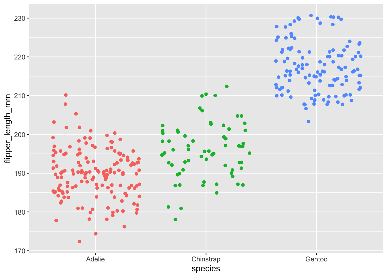
Here, the factor is the species variable which contains 3 modalities or groups (Adelie, Chinstrap and Gentoo).
Aim and hypotheses of ANOVA
As mentioned in the introduction, the ANOVA is used to compare groups (in practice, 3 or more groups). More generally, it is used to:
- study whether measurements are similar across different modalities (also called levels or treatments in the context of ANOVA) of a categorical variable
- compare the impact of the different levels of a categorical variable on a quantitative variable
- explain a quantitative variable based on a qualitative variable
In this context and as an example, we are going to use an ANOVA to help us answer the question: “Is the length of the flippers different between the 3 species of penguins?”.
The null and alternative hypothesis of an ANOVA are:
- \(H_0\): \(\mu_{Adelie} = \mu_{Chinstrap} = \mu_{Gentoo}\) (\(\Rightarrow\) the 3 species are equal in terms of flipper length)
- \(H_1\): at least one mean is different (\(\Rightarrow\) at least one species is different from the other 2 species in terms of flipper length)
Be careful that the alternative hypothesis is not that all means are different. The opposite of all means being equal (\(H_0\)) is that at least one mean is different from the others (\(H_1\)).
In this sense, if the null hypothesis is rejected, it means that at least one species is different from the other 2, but not necessarily that all 3 species are different from each other. It could be that flipper length for the species Gentoo is different than for the species Chinstrap and Adelie, but flipper length is similar between Chinstrap and Adelie. Other types of test (known as post-hoc tests and covered in this section) must be performed to test whether all 3 species differ.
Underlying assumptions of ANOVA
As for many statistical tests, there are some assumptions that need to be met in order to be able to interpret the results. When one or several assumptions are not met, although it is technically possible to perform these tests, it would be incorrect to interpret the results and trust the conclusions.
Below are the assumptions of the ANOVA, how to test them and which other tests exist if an assumption is not met:
- Variable type: ANOVA requires a mix of one continuous quantitative dependent variable (which corresponds to the measurements to which the question relates) and one qualitative independent variable (with at least 2 levels which will determine the groups to compare).
- Independence: the data, collected from a representative and randomly selected portion of the total population, should be independent between groups and within each group. The assumption of independence is most often verified based on the design of the experiment and on the good control of experimental conditions rather than via a formal test. If you are still unsure about independence based on the experiment design, ask yourself if one observation is related to another (if one observation has an impact on another) within each group or between the groups themselves. If not, it is most likely that you have independent samples. If observations between samples (forming the different groups to be compared) are dependent (for example, if three measurements have been collected on the same individuals as it is often the case in medical studies when measuring a metric (i) before, (ii) during and (iii) after a treatment), the repeated measures ANOVA should be preferred in order to take into account the dependency between the samples.
- Normality:
- In case of small samples, residuals2 should follow approximately a normal distribution. The normality assumption can be tested visually thanks to a histogram and a QQ-plot, and/or formally via a normality test such as the Shapiro-Wilk or Kolmogorov-Smirnov test. If, even after a transformation of your data (e.g., logarithmic transformation, square root, Box-Cox, etc.), the residuals still do not follow approximately a normal distribution, the Kruskal-Wallis test can be applied (
kruskal.test(variable ~ group, data = datin R). This non-parametric test, robust to non normal distributions, has the same goal than the ANOVA—compare 3 or more groups—but it uses sample medians instead of sample means to compare groups. - In case of large samples, normality is not required (this is a common misconception!). By the central limit theorem, sample means of large samples are often well-approximated by a normal distribution even if the data are not normally distributed (Stevens 2013).3 It is therefore not required to test the normality assumption when the number of observations in each group/sample is large (usually \(n \ge 30\)).
- In case of small samples, residuals2 should follow approximately a normal distribution. The normality assumption can be tested visually thanks to a histogram and a QQ-plot, and/or formally via a normality test such as the Shapiro-Wilk or Kolmogorov-Smirnov test. If, even after a transformation of your data (e.g., logarithmic transformation, square root, Box-Cox, etc.), the residuals still do not follow approximately a normal distribution, the Kruskal-Wallis test can be applied (
- Equality of variances: the variances of the different groups should be equal in the populations (an assumption called homogeneity of the variances, or even sometimes referred as homoscedasticity, as opposed to heteroscedasticity if variances are different across groups). This assumption can be tested graphically (by comparing the dispersion in a boxplot or dotplot for instance), or more formally via the Levene’s test (
leveneTest(variable ~ group)from the{car}package) or Bartlett’s test, among others. If the hypothesis of equal variances is rejected, another version of the ANOVA can be used: the Welch ANOVA (oneway.test(variable ~ group, var.equal = FALSE)). Note that the Welch ANOVA does not require homogeneity of the variances, but the distributions should still follow approximately a normal distribution. Note that the Kruskal-Wallis test does not require the assumptions of normality nor homoscedasticity of the variances.4 - Outliers: An outlier is a value or an observation that is distant from the other observations. There should be no significant outliers in the different groups, or the conclusions of your ANOVA may be flawed. There are several methods to detect outliers in your data but in order to deal with them, it is your choice to either:
- use the non-parametric version (i.e., the Kruskal-Wallis test)
- transform your data (logarithmic or Box-Cox transformation, among others)
- or remove them (be careful)
Choosing the appropriate test depending on whether assumptions are met may be confusing so here is a brief summary:
- Check that your observations are independent.
- Sample sizes:
- In case of small samples, test the normality of residuals:
- If normality is assumed, test the homogeneity of the variances:
- If variances are equal, use ANOVA.
- If variances are not equal, use the Welch ANOVA.
- If normality is not assumed, use the Kruskal-Wallis test.
- If normality is assumed, test the homogeneity of the variances:
- In case of large samples normality is assumed, so test the homogeneity of the variances:
- If variances are equal, use ANOVA.
- If variances are not equal, use the Welch ANOVA.
- In case of small samples, test the normality of residuals:
Now that we have seen the underlying assumptions of the ANOVA, we review them specifically for our dataset before applying the appropriate version of the test.
Variable type
The dependent variable flipper_length_mm is a quantitative variable and the independent variable species is a qualitative one (with 3 levels corresponding to the 3 species). So we have a mix of the two types of variable and this assumption is met.
Independence
Independence of the observations is assumed as data have been collected from a randomly selected portion of the population and measurements within and between the 3 samples are not related.
The independence assumption is most often verified based on the design of the experiment and on the good control of experimental conditions, as it is the case here.
If you really want to test it more formally, you can, however, test it via a statistical test—the Durbin-Watson test (in R: durbinWatsonTest(res_lm) where res_lm is a linear model). The null hypothesis of this test specifies an autocorrelation coefficient = 0, while the alternative hypothesis specifies an autocorrelation coefficient \(\ne\) 0.
Normality
Since the smallest sample size per group (i.e., per species) is 68, we have large samples. Therefore, we do not need to check normality.
Usually, we would directly test the homogeneity of the variances without testing normality. However, for the sake of illustration, we act as if the sample sizes were small in order to illustrate what would need to be done in that case.
Remember that normality of residuals can be tested visually via a histogram and a QQ-plot, and/or formally via a normality test (Shapiro-Wilk test for instance).
Before checking the normality assumption, we first need to compute the ANOVA (more on that in this section). We then save the results in res_aov :
res_aov <- aov(flipper_length_mm ~ species,
  data = dat
)
We can now check normality visually:
par(mfrow = c(1, 2)) # combine plots

# histogram
hist(res_aov$residuals)

# QQ-plot
library(car)
qqPlot(res_aov$residuals,
  id = FALSE # id = FALSE to remove point identification
)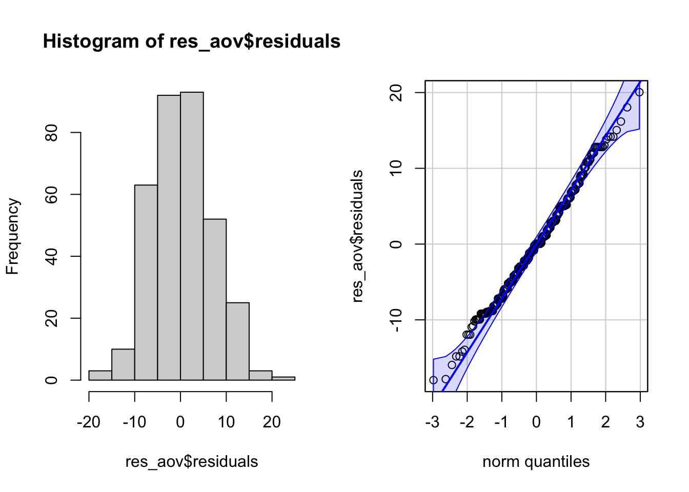
From the histogram and QQ-plot above, we can already see that the normality assumption seems to be met. Indeed, the histogram roughly form a bell curve, indicating that the residuals follow a normal distribution. Furthermore, points in the QQ-plots roughly follow the straight line and most of them are within the confidence bands, also indicating that residuals follow approximately a normal distribution.
Some researchers stop here and assume that normality is met, while others also test the assumption via a formal normality test. It is your choice to test it (i) only visually, (ii) only via a normality test, or (iii) both visually AND via a normality test. Bear in mind, however, the two following points:
- ANOVA is quite robust to small deviations from normality. This means that it is not an issue (from the perspective of the interpretation of the ANOVA results) if a small number of points deviates slightly from the normality,
- normality tests are sometimes quite conservative, meaning that the null hypothesis of normality may be rejected due to a limited deviation from normality. This is especially the case with large samples as power of the test increases with the sample size.
In practice, I tend to prefer the (i) visual approach only, but again, this is a matter of personal choice and also depends on the context of the analysis.
Still for the sake of illustration, we also now test the normality assumption via a normality test. You can use the Shapiro-Wilk test or the Kolmogorov-Smirnov test, among others.
Remember that the null and alternative hypothesis of these tests are:
- \(H_0\): data come from a normal distribution
- \(H_1\): data do not come from a normal distribution
In R, we can test normality of the residuals with the Shapiro-Wilk test thanks to the shapiro.test() function:
shapiro.test(res_aov$residuals)##
## Shapiro-Wilk normality test
##
## data: res_aov$residuals
## W = 0.99452, p-value = 0.2609P-value of the Shapiro-Wilk test on the residuals is larger than the usual significance level of \(\alpha = 5\%\), so we do not reject the hypothesis that residuals follow a normal distribution (p-value = 0.261).
This result is in line with the visual approach. In our case, the normality assumption is thus met both visually and formally.
Side note: Remind that the p-value is the probability of having observations as extreme as the ones we have observed in the sample(s) given that the null hypothesis is true. If the p-value \(< \alpha\) (indicating that it is not likely to observe the data we have in the sample given that the null hypothesis is true), the null hypothesis is rejected, otherwise the null hypothesis is not rejected. See more about p-value and significance level if you are unfamiliar with those important statistical concepts.
Remember that if the normality assumption was not reached, some transformation(s) would need to be applied on the raw data in the hope that residuals would better fit a normal distribution, or you would need to use the non-parametric version of the ANOVA—the Kruskal-Wallis test.
As pointed out by a reader (see comments at the very end of the article), the normality assumption can also be tested on the “raw” data (i.e., the observations) instead of the residuals. However, if you test the normality assumption on the raw data, it must be tested for each group separately as the ANOVA requires normality in each group.
Testing normality on all residuals or on the observations per group is equivalent, and will give similar results. Indeed, saying “The distribution of Y within each group is normally distributed” is the same as saying “The residuals are normally distributed”.
Remember that residuals are the distance between the actual value of Y and the mean value of Y for a specific value of X, so the grouping variable is induced in the computation of the residuals.
So in summary, in ANOVA you actually have two options for testing normality:
- Checking normality separately for each group on the “raw” data (Y values)
- Checking normality on all residuals (but not per group)
In practice, you will see that it is often easier to just use the residuals and check them all together, especially if you have many groups or few observations per group.
If you are still not convinced: remember that an ANOVA is a special case of a linear model. Suppose your independent variable is a continuous variable (instead of a categorical variable), the only option you have left is to check normality on the residuals, which is precisely what is done for testing normality in linear regression models.
Equality of variances - homogeneity
Assuming residuals follow a normal distribution, it is now time to check whether the variances are equal across species or not. The result will have an impact on whether we use the ANOVA or the Welch ANOVA.
This can again be verified visually—via a boxplot or dotplot—or more formally via a statistical test (Levene’s test, among others).
Visually, we have:
# Boxplot
boxplot(flipper_length_mm ~ species,
  data = dat
)
# Dotplot
library("lattice")

dotplot(flipper_length_mm ~ species,
  data = dat
)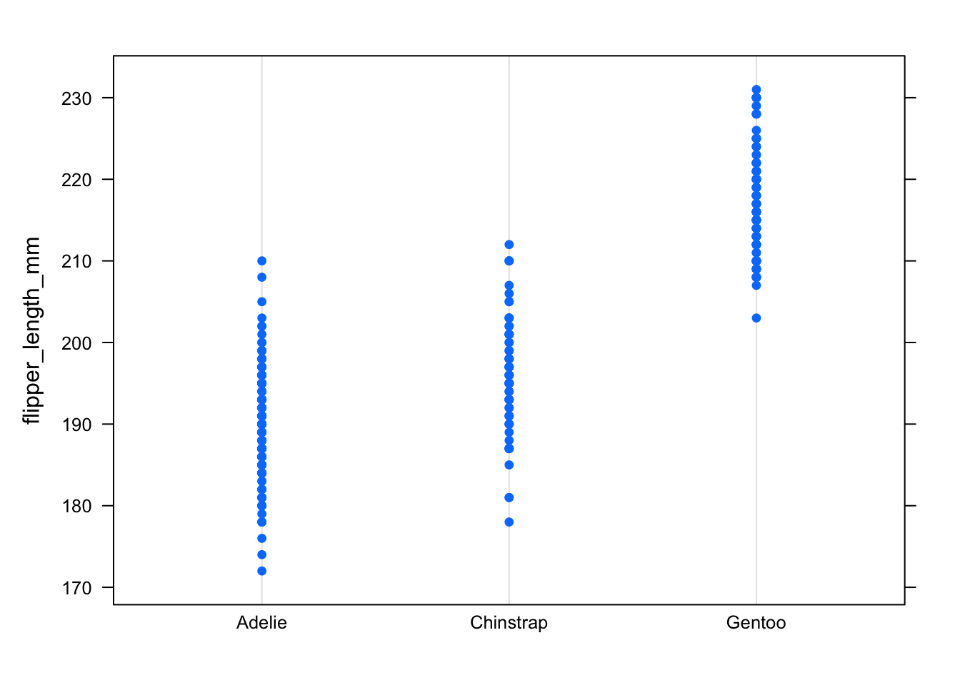
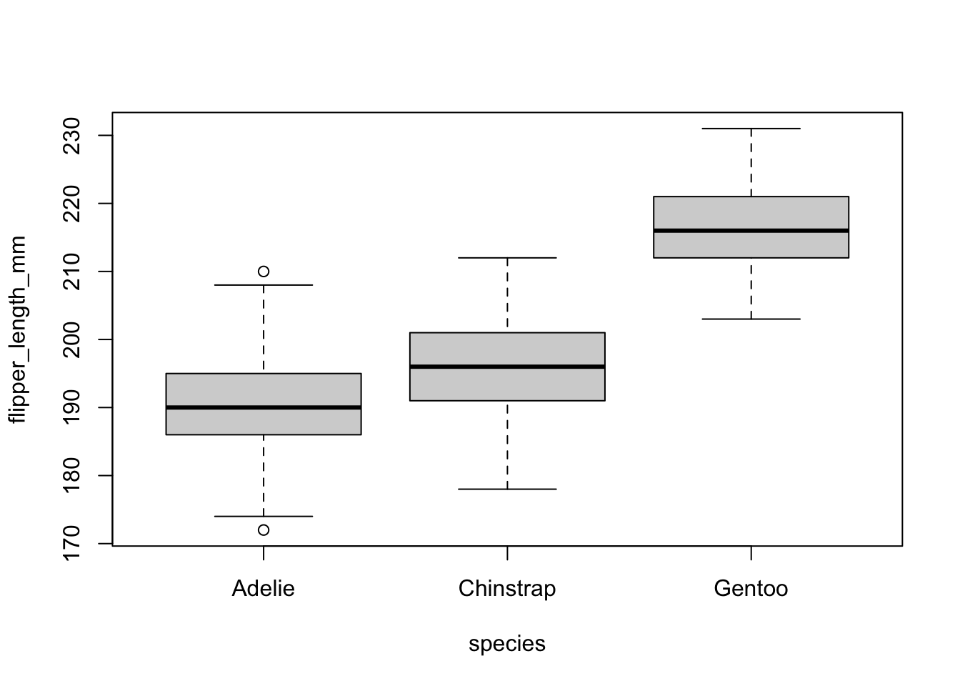
Both the boxplot and the dotplot show a similar variance for the different species. In the boxplot, this can be seen by the fact that the boxes and the whiskers have a comparable size for all species.
There are a couple of outliers as shown by the points outside the whiskers, but this does not change the fact that the dispersion is more or less the same between the different species.
In the dotplot, this can be seen by the fact that points for all 3 species have more or less the same range, a sign of the dispersion and thus the variance being similar.
Like the normality assumption, if you feel that the visual approach is not sufficient, you can formally test for equality of the variances with a Levene’s or Bartlett’s test. Notice that the Levene’s test is less sensitive to departures from normal distribution than the Bartlett’s test.
The null and alternative hypothesis for both tests are:
- \(H_0\): variances are equal
- \(H_1\): at least one variance is different
In R, the Levene’s test can be performed thanks to the leveneTest() function from the {car} package:
# Levene's test
library(car)

leveneTest(flipper_length_mm ~ species,
  data = dat
)
## Levene's Test for Homogeneity of Variance (center = median)
## Df F value Pr(>F)
## group 2 0.3306 0.7188
## 339The p-value being larger than the significance level of 0.05, we do not reject the null hypothesis, so we cannot reject the hypothesis that variances are equal between species (p-value = 0.719).
This result is also in line with the visual approach, so the homogeneity of variances is met both visually and formally.
Another method to test normality and homogeneity
For your information, it is also possible to test the homogeneity of the variances and the normality of the residuals visually (and both at the same time) via the plot() function:
par(mfrow = c(1, 2)) # combine plots

# 1. Homogeneity of variances
plot(res_aov, which = 3)

# 2. Normality
plot(res_aov, which = 2)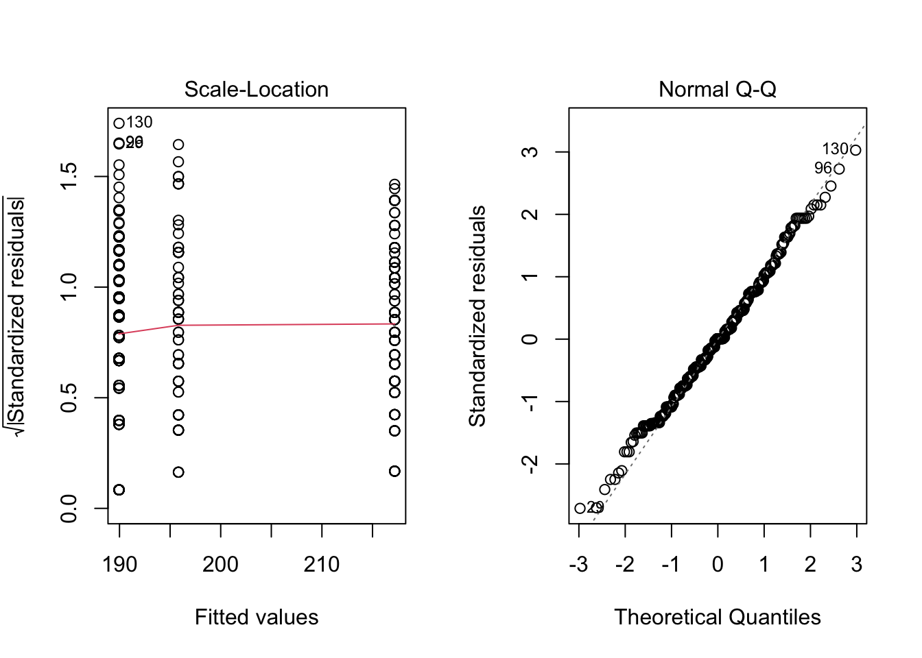
Plot on the left hand side shows that there is no evident relationships between residuals and fitted values (the mean of each group), so homogeneity of variances is assumed. If homogeneity of variances was violated, the red line would not be flat (horizontal).
Plot on the right hand side shows that residuals follow approximately a normal distribution, so normality is assumed. If normality was violated, points would consistently deviate from the dashed line.
Outliers
There are several techniques to detect outliers. In this article, we focus on the most simple one (yet very efficient)—the visual approach via a boxplot:
boxplot(flipper_length_mm ~ species,
  data = dat
)
There is one outlier in the group Adelie, as defined by the interquartile range criterion. This point is, however, not seen as a significant outlier so we can assume that the assumption of no significant outliers is met.
ANOVA
We showed that all assumptions of the ANOVA are met.
We can thus proceed to the implementation of the ANOVA in R, but first, let’s do some preliminary analyses to better understand the research question.
Preliminary analyses
A good practice before actually performing the ANOVA in R is to visualize the data in relation to the research question. The best way to do so is to draw and compare boxplots of the quantitative variable flipper_length_mm for each species.
This can be done with the boxplot() function in base R (same code than the visual check of equal variances):
boxplot(flipper_length_mm ~ species,
  data = dat
)
Or with the {ggplot2} package:
library(ggplot2)

ggplot(dat) +
  aes(x = species, y = flipper_length_mm) +
  geom_boxplot()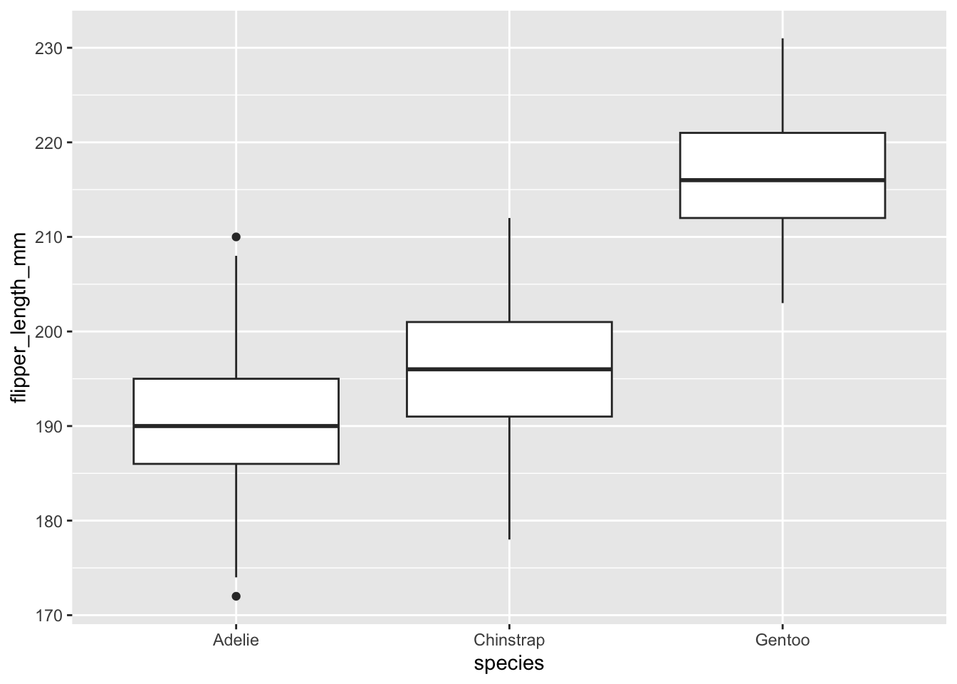
The boxplots above show that, at least for our sample, penguins of the species Gentoo seem to have the biggest flipper, and Adelie species the smallest flipper.
Besides a boxplot for each species, it is also a good practice to compute some descriptive statistics such as the mean and standard deviation by species.
This can be done, for instance, with the aggregate() function:
aggregate(flipper_length_mm ~ species,
  data = dat,
  function(x) round(c(mean = mean(x), sd = sd(x)), 2)
)
## species flipper_length_mm.mean flipper_length_mm.sd
## 1 Adelie 189.95 6.54
## 2 Chinstrap 195.82 7.13
## 3 Gentoo 217.19 6.48or with the summarise() and group_by() functions from the {dplyr} package:
library(dplyr)

group_by(dat, species) %>%
  summarise(
    mean = mean(flipper_length_mm, na.rm = TRUE),
    sd = sd(flipper_length_mm, na.rm = TRUE)
  )
## # A tibble: 3 × 3
## species mean sd
## <fct> <dbl> <dbl>
## 1 Adelie 190. 6.54
## 2 Chinstrap 196. 7.13
## 3 Gentoo 217. 6.48Mean is also the lowest for Adelie and highest for Gentoo. Boxplots and descriptive statistics are, however, not enough to conclude that flippers are significantly different in the 3 populations of penguins.
ANOVA in R
As you guessed by now, only the ANOVA can help us to make inference about the population given the sample at hand, and help us to answer the initial research question “Is the length of the flippers different between the 3 species of penguins?”.
ANOVA in R can be done in several ways, of which two are presented below:
- With the
oneway.test()function:
# 1st method:
oneway.test(flipper_length_mm ~ species,
  data = dat,
  var.equal = TRUE # assuming equal variances
)
##
## One-way analysis of means
##
## data: flipper_length_mm and species
## F = 594.8, num df = 2, denom df = 339, p-value < 2.2e-16- With the
summary()andaov()functions:
# 2nd method:
res_aov <- aov(flipper_length_mm ~ species,
  data = dat
)

summary(res_aov)
## Df Sum Sq Mean Sq F value Pr(>F)
## species 2 52473 26237 594.8 <2e-16 ***
## Residuals 339 14953 44
## ---
## Signif. codes: 0 '***' 0.001 '**' 0.01 '*' 0.05 '.' 0.1 ' ' 1
## 2 observations deleted due to missingnessAs you can see from the two outputs above, the test statistic (F = in the first method and F value in the second one) and the p-value (p-value in the first method and Pr(>F) in the second one) are exactly the same for both methods, which means that in case of equal variances, results and conclusions will be unchanged.
The advantage of the first method is that it is easy to switch from the ANOVA (used when variances are equal) to the Welch ANOVA (used when variances are unequal). This can be done by replacing var.equal = TRUE by var.equal = FALSE, as presented below:
oneway.test(flipper_length_mm ~ species,
  data = dat,
  var.equal = FALSE # assuming unequal variances
)
##
## One-way analysis of means (not assuming equal variances)
##
## data: flipper_length_mm and species
## F = 614.01, num df = 2.00, denom df = 172.76, p-value < 2.2e-16The advantage of the second method, however, is that:
- the full ANOVA table (with degrees of freedom, mean squares, etc.) is printed, which may be of interest in some (theoritical) cases
- results of the ANOVA (
res_aov) can be saved for later use (especially useful for post-hoc tests)
Interpretations of ANOVA results
Given that the p-value is smaller than 0.05, we reject the null hypothesis, so we reject the hypothesis that all means are equal. Therefore, we can conclude that at least one species is different than the others in terms of flippers length (p-value < 2.2e-16).
(For the sake of illustration, if the p-value was larger than 0.05: we cannot reject the null hypothesis that all means are equal, so we cannot reject the hypothesis that the 3 considered species of penguins are equal in terms of flippers length.)
A nice and easy way to report results of an ANOVA in R is with the report() function from the {report} package:
# install.packages("remotes")
# remotes::install_github("easystats/report") # You only need to do that once
library("report") # Load the package every time you start R

report(res_aov)
## The ANOVA (formula: flipper_length_mm ~ species) suggests that:
##
## - The main effect of species is statistically significant and large (F(2, 339)
## = 594.80, p < .001; Eta2 = 0.78, 95% CI [0.75, 1.00])
##
## Effect sizes were labelled following Field's (2013) recommendations.As you can see, the function interprets the results for you and indicates a large and significant main effect of the species on the flipper length (p-value < .001).
Note that the report() function can be used for other analyses. See more tips and tricks in R if you find this one useful.
What’s next?
If the null hypothesis is not rejected (p-value \(\ge\) 0.05), it means that we do not reject the hypothesis that all groups are equal. The ANOVA more or less stops here.
Other types of analyses can be performed of course, but—given the data at hand—we could not prove that at least one group was different so we usually do not go further with the ANOVA.
On the contrary, if the null hypothesis is rejected (as it is our case since the p-value < 0.05), we proved that at least one group is different. We can decide to stop here if we are only interested to test whether all species are equal in terms of flippers length.
But most of the time, when we showed thanks to an ANOVA that at least one group is different, we are also interested in knowing which one(s) is(are) different. Results of an ANOVA, however, do NOT tell us which group(s) is(are) different from the others.
To test this, we need to use other types of test, referred as post-hoc tests (in Latin, “after this”, so after obtaining statistically significant ANOVA results) or multiple pairwise-comparison tests.5
This family of statistical tests is the topic of the following sections.
Post-hoc test
Issue of multiple testing
In order to see which group(s) is(are) different from the others, we need to compare groups 2 by 2. In practice, since there are 3 species, we are going to compare species 2 by 2 as follows:
- Chinstrap versus Adelie
- Gentoo vs. Adelie
- Gentoo vs. Chinstrap
In theory, we could compare species thanks to 3 Student’s t-tests since we need to compare 2 groups and a t-test is used precisely in that case.
However, if several t-tests are performed, the issue of multiple testing (also referred as multiplicity) arises. In short, when several statistical tests are performed, some will have p-values less than \(\alpha\) purely by chance, even if all null hypotheses are in fact true.
To demonstrate the problem, consider our case where we have 3 hypotheses to test and a desired significance level of 0.05.
The probability of observing at least one significant result (at least one p-value < 0.05) just due to chance is:
\[\begin{equation} \begin{split} P(\text{at least 1 sig. result}) & = 1 - P(\text{no sig. results}) \\ & = 1 - (1 - 0.05)^3 \\ & = 0.142625 \end{split} \end{equation}\]
So, with as few as 3 tests being considered, we already have a 14.26% chance of observing at least one significant result, even if all of the tests are actually not significant.
And as the number of groups increases, the number of comparisons increases as well, so the probability of having a significant result simply due to chance keeps increasing.
For example, with 10 groups we need to make 45 comparisons and the probability of having at least one significant result by chance becomes \(1 - (1 - 0.05)^{45} = 90\%\). So it is very likely to observe a significant result just by chance when comparing 10 groups, and when we have 14 groups or more we are almost certain (99%) to have a false positive!
Post-hoc tests take into account that multiple tests are done and deal with the problem by adjusting \(\alpha\) in some way, so that the probability of observing at least one significant result due to chance remains below our desired significance level.6
Post-hoc tests in R and their interpretation
Post-hoc tests are a family of statistical tests so there are several of them. The most common ones are:
- Tukey HSD, used to compare all groups to each other (so all possible comparisons of 2 groups).
- Dunnett, used to make comparisons with a reference group. For example, consider 2 treatment groups and one control group. If you only want to compare the 2 treatment groups with respect to the control group, and you do not want to compare the 2 treatment groups to each other, the Dunnett’s test is preferred.
- Bonferroni correction if one has a set of planned comparisons to do.
The Bonferroni correction is simple: you simply divide the desired global \(\alpha\) level by the number of comparisons.
In our example, we have 3 comparisons so if we want to keep a global \(\alpha = 0.05\), we have \(\alpha' = \frac{0.05}{3} = 0.0167\). We can then simply perform a Student’s t-test for each comparison, and compare the obtained \(p\)-values with this new \(\alpha'\).
The other two post-hoc tests are presented in the next sections.
Note that variances are assumed to be equal for all three methods (unless you use the Welch’s t-test instead of the Student’s t-test with the Bonferroni correction). If variances are not equal, you can use the Games-Howell test, among others.
Tukey HSD test
In our case, since there is no “reference” species and we are interested in comparing all species, we are going to use the Tukey HSD test.
In R, the Tukey HSD test is done as follows. This is where the second method to perform the ANOVA comes handy because the results (res_aov) are reused for the post-hoc test:
library(multcomp)

# Tukey HSD test:
post_test <- glht(res_aov,
  linfct = mcp(species = "Tukey")
)

summary(post_test)
##
## Simultaneous Tests for General Linear Hypotheses
##
## Multiple Comparisons of Means: Tukey Contrasts
##
##
## Fit: aov(formula = flipper_length_mm ~ species, data = dat)
##
## Linear Hypotheses:
## Estimate Std. Error t value Pr(>|t|)
## Chinstrap - Adelie == 0 5.8699 0.9699 6.052 1.03e-08 ***
## Gentoo - Adelie == 0 27.2333 0.8067 33.760 < 1e-08 ***
## Gentoo - Chinstrap == 0 21.3635 1.0036 21.286 < 1e-08 ***
## ---
## Signif. codes: 0 '***' 0.001 '**' 0.01 '*' 0.05 '.' 0.1 ' ' 1
## (Adjusted p values reported -- single-step method)In the output of the Tukey HSD test, we are interested in the table displayed after Linear Hypotheses:, and more precisely, in the first and last column of the table. The first column shows the comparisons which have been made; the last column (Pr(>|t|)) shows the adjusted7 p-values for each comparison (with the null hypothesis being the two groups are equal and the alternative hypothesis being the two groups are different).
It is these adjusted p-values that are used to test whether two groups are significantly different or not, and we can be confident that the entire set of comparisons collectively has an error rate of 0.05.
In our example, we tested:
- Chinstrap versus Adelie (line
Chinstrap - Adelie == 0) - Gentoo vs. Adelie (line
Gentoo - Adelie == 0) - Gentoo vs. Chinstrap (line
Gentoo - Chinstrap == 0)
All three ajusted p-values are smaller than 0.05, so we reject the null hypothesis for all comparisons, which means that all species are significantly different in terms of flippers length.
The results of the post-hoc test can be visualized with the plot() function:
par(mar = c(3, 8, 3, 3))
plot(post_test)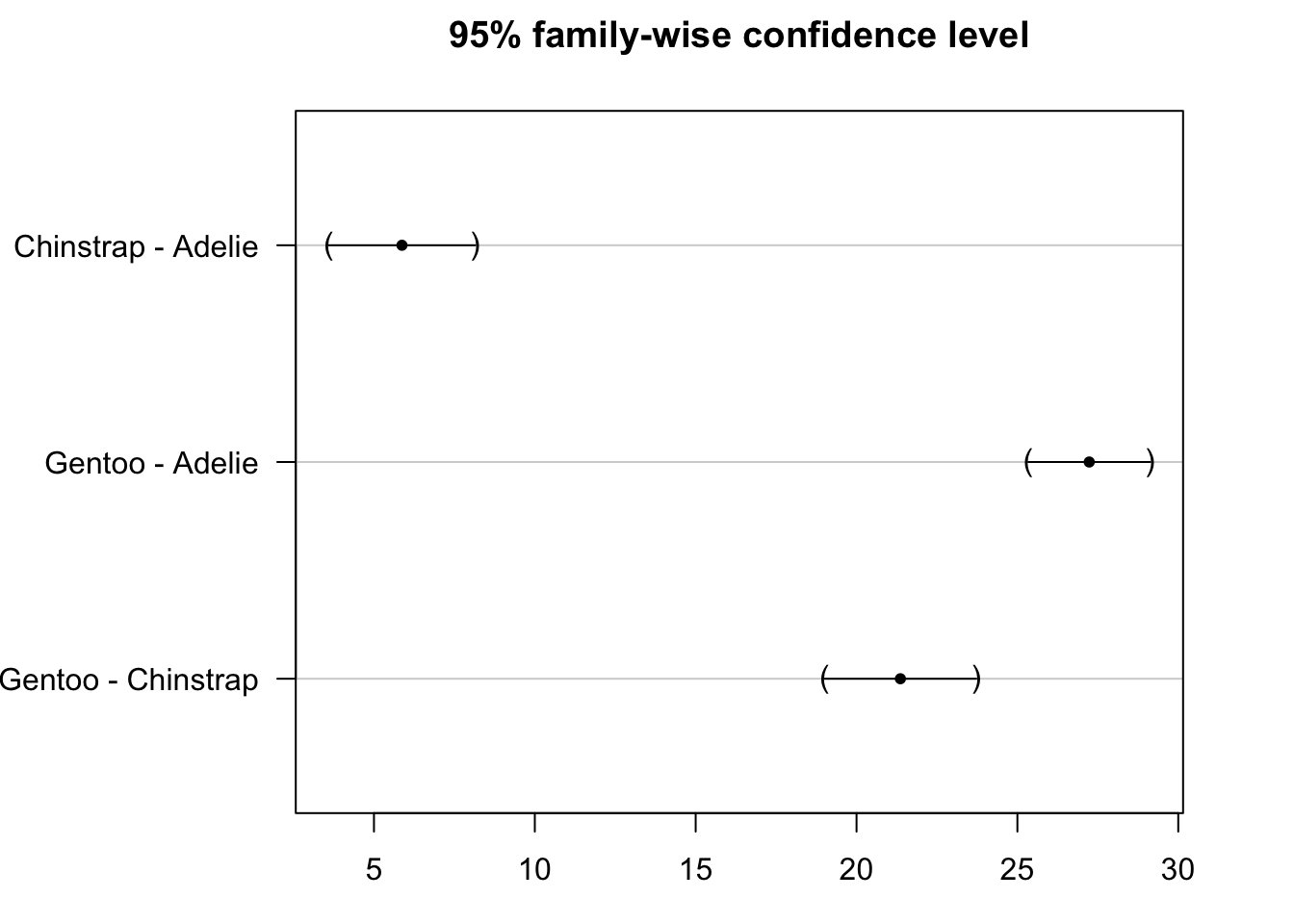
We see that the confidence intervals do not cross the zero line, which indicate that all groups are significantly different.
Note that the Tukey HSD test can also be done in R with the TukeyHSD() function:
TukeyHSD(res_aov)## Tukey multiple comparisons of means
## 95% family-wise confidence level
##
## Fit: aov(formula = flipper_length_mm ~ species, data = dat)
##
## $species
## diff lwr upr p adj
## Chinstrap-Adelie 5.869887 3.586583 8.153191 0
## Gentoo-Adelie 27.233349 25.334376 29.132323 0
## Gentoo-Chinstrap 21.363462 19.000841 23.726084 0With this code, it is the column p adj (also the last column) which is of interest. Notice that the conclusions are the same than above: all species are significantly different in terms of flippers length.
The results can also be visualized with the plot() function:
plot(TukeyHSD(res_aov))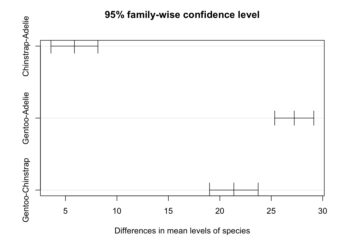
Dunnett’s test
We have seen in this section that as the number of groups increases, the number of comparisons also increases. And as the number of comparisons increases, the post-hoc analysis must lower the individual significance level even further, which leads to lower statistical power (so a difference between group means in the population is less likely to be detected).
One method to mitigate this and increase the statistical power is by reducing the number of comparisons. This reduction allows the post-hoc procedure to use a larger individual error rate to achieve the desired global error rate.
While comparing all possible groups with a Tukey HSD test is a common approach, many studies have a control group and several treatment groups. For these studies, you may need to compare the treatment groups only to the control group, which reduces the number of comparisons.
Dunnett’s test does precisely this—it only compares a group taken as reference to all other groups, but it does not compare all groups to each others.
So to recap:
- the Tukey HSD test allows to compares all groups but at the cost of less power
- the Dunnett’s test allows to only make comparisons with a reference group, but with the benefit of more power
Now, again for the sake of illustration, consider that the species Adelie is the reference species and we are only interested in comparing the reference species against the other 2 species. In that scenario, we would use the Dunnett’s test.
In R, the Dunnett’s test is done as follows (the only difference with the code for the Tukey HSD test is in the line linfct = mcp(species = "Dunnett")):
library(multcomp)

# Dunnett's test:
post_test <- glht(res_aov,
  linfct = mcp(species = "Dunnett")
)

summary(post_test)
##
## Simultaneous Tests for General Linear Hypotheses
##
## Multiple Comparisons of Means: Dunnett Contrasts
##
##
## Fit: aov(formula = flipper_length_mm ~ species, data = dat)
##
## Linear Hypotheses:
## Estimate Std. Error t value Pr(>|t|)
## Chinstrap - Adelie == 0 5.8699 0.9699 6.052 7.59e-09 ***
## Gentoo - Adelie == 0 27.2333 0.8067 33.760 < 1e-10 ***
## ---
## Signif. codes: 0 '***' 0.001 '**' 0.01 '*' 0.05 '.' 0.1 ' ' 1
## (Adjusted p values reported -- single-step method)The interpretation is the same as for the Tukey HSD test’s except that in the Dunett’s test we only compare:
- Chinstrap versus Adelie (line
Chinstrap - Adelie == 0) - Gentoo vs. Adelie (line
Gentoo - Adelie == 0)
Both adjusted p-values (displayed in the last column) are below 0.05, so we reject the null hypothesis for both comparisons.
This means that both the species Chinstrap and Gentoo are significantly different from the reference species Adelie in terms of flippers length. (Nothing can be said about the comparison between Chinstrap and Gentoo though.)
Again, the results of the post-hoc test can be visualized with the plot() function:
par(mar = c(3, 8, 3, 3))
plot(post_test)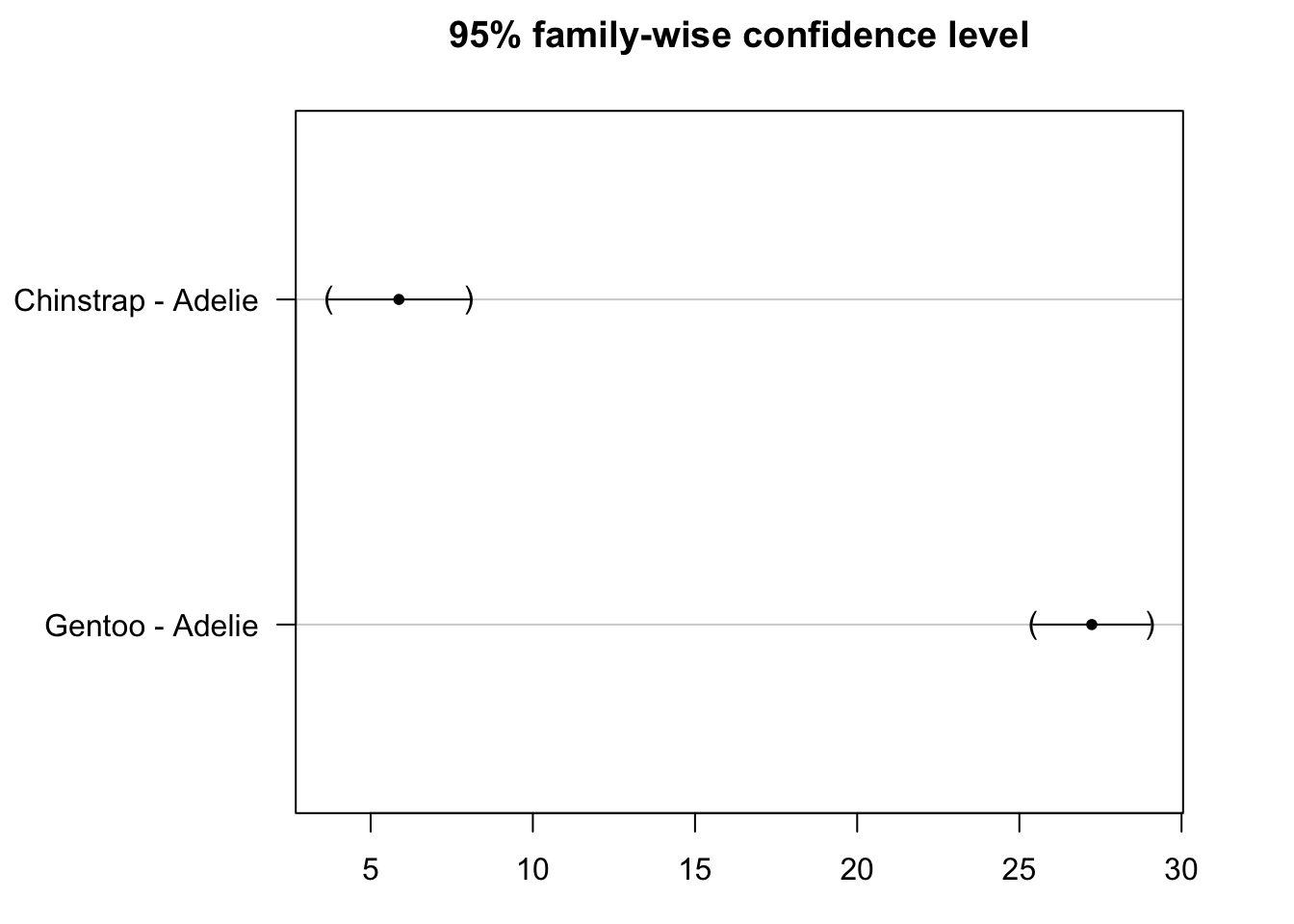
We see that the confidence intervals do not cross the zero line, which indicate that both the species Gentoo and Chinstrap are significantly different from the reference species Adelie.
Note that in R, by default, the reference category for a factor variable is the first category in alphabetical order. This is the reason that, by default, the reference species is Adelie.
The reference category can be changed with the relevel() function (or with the {questionr} addin). Considering that we want Gentoo as the reference category instead of Adelie:
# Change reference category:
dat$species <- relevel(dat$species, ref = "Gentoo")

# Check that Gentoo is the reference category:
levels(dat$species)
## [1] "Gentoo" "Adelie" "Chinstrap"Gentoo now being the first category of the three, it is indeed considered as the reference level.
In order to perform the Dunnett’s test with the new reference we first need to rerun the ANOVA to take into account the new reference:
res_aov2 <- aov(flipper_length_mm ~ species,
  data = dat
)
We can then run the Dunett’s test with the new results of the ANOVA:
# Dunnett's test:
post_test <- glht(res_aov2,
  linfct = mcp(species = "Dunnett")
)

summary(post_test)
##
## Simultaneous Tests for General Linear Hypotheses
##
## Multiple Comparisons of Means: Dunnett Contrasts
##
##
## Fit: aov(formula = flipper_length_mm ~ species, data = dat)
##
## Linear Hypotheses:
## Estimate Std. Error t value Pr(>|t|)
## Adelie - Gentoo == 0 -27.2333 0.8067 -33.76 <1e-10 ***
## Chinstrap - Gentoo == 0 -21.3635 1.0036 -21.29 <1e-10 ***
## ---
## Signif. codes: 0 '***' 0.001 '**' 0.01 '*' 0.05 '.' 0.1 ' ' 1
## (Adjusted p values reported -- single-step method)par(mar = c(3, 8, 3, 3))
plot(post_test)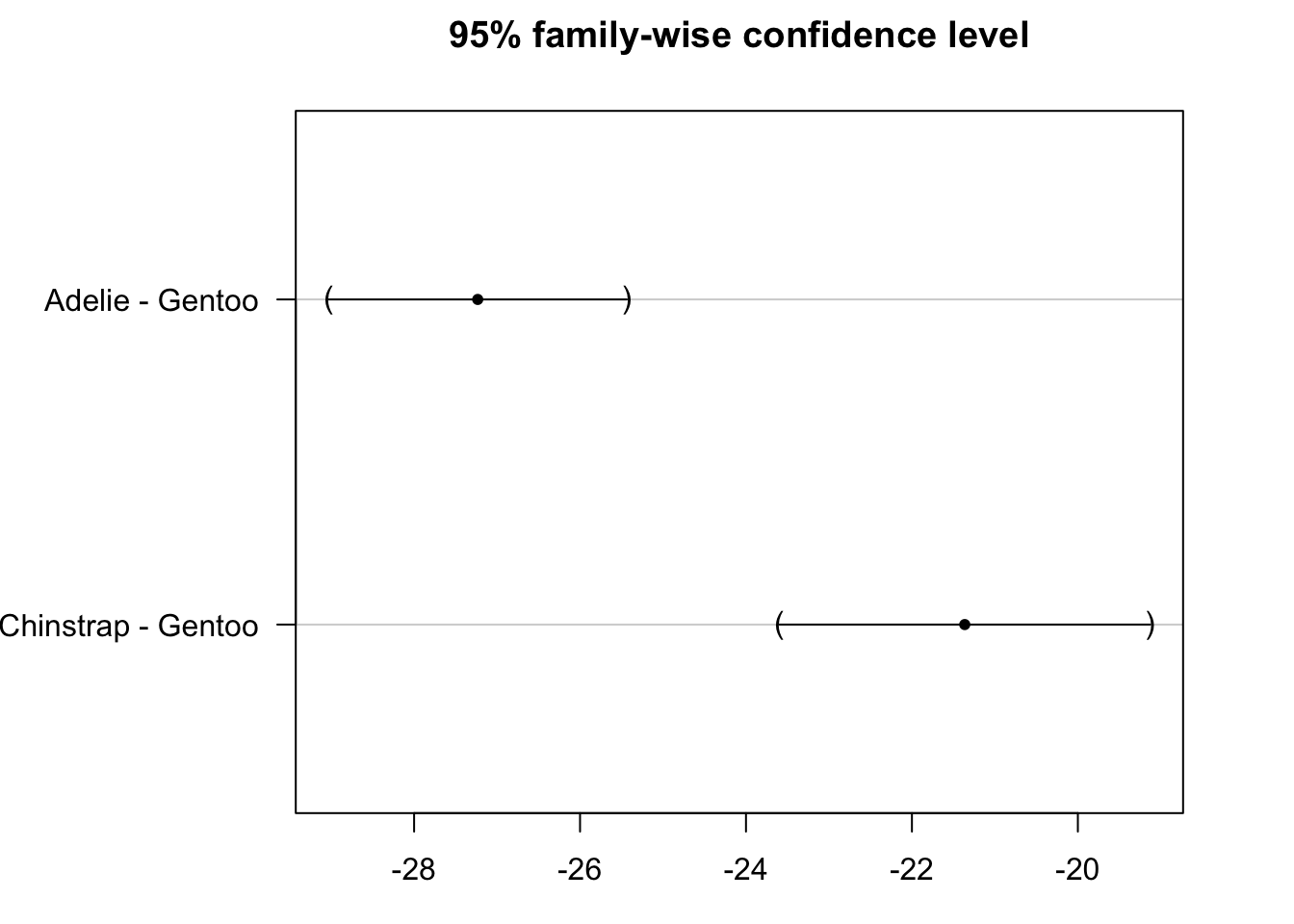
From the results above we conclude that Adelie and Chinstrap species are significantly different from Gentoo species in terms of flippers length (adjusted p-values < 1e-10).
Note that even if your study does not have a reference group which you can compare to the other groups, it is still often better to do multiple comparisons determined by some research questions than to do all-pairwise tests. By reducing the number of post-hoc comparisons to what is necessary only, and no more, you maximize the statistical power.8
Other p-values adjustment methods
For the interested readers, note that you can use other p-values adjustment methods by using the pairwise.t.test() function:
pairwise.t.test(dat$flipper_length_mm, dat$species,
  p.adjust.method = "holm"
)
##
## Pairwise comparisons using t tests with pooled SD
##
## data: dat$flipper_length_mm and dat$species
##
## Gentoo Adelie
## Adelie < 2e-16 -
## Chinstrap < 2e-16 3.8e-09
##
## P value adjustment method: holmBy default, the Holm method is applied but other methods exist. See ?p.adjust for all available options.
Visualization of ANOVA and post-hoc tests on the same plot
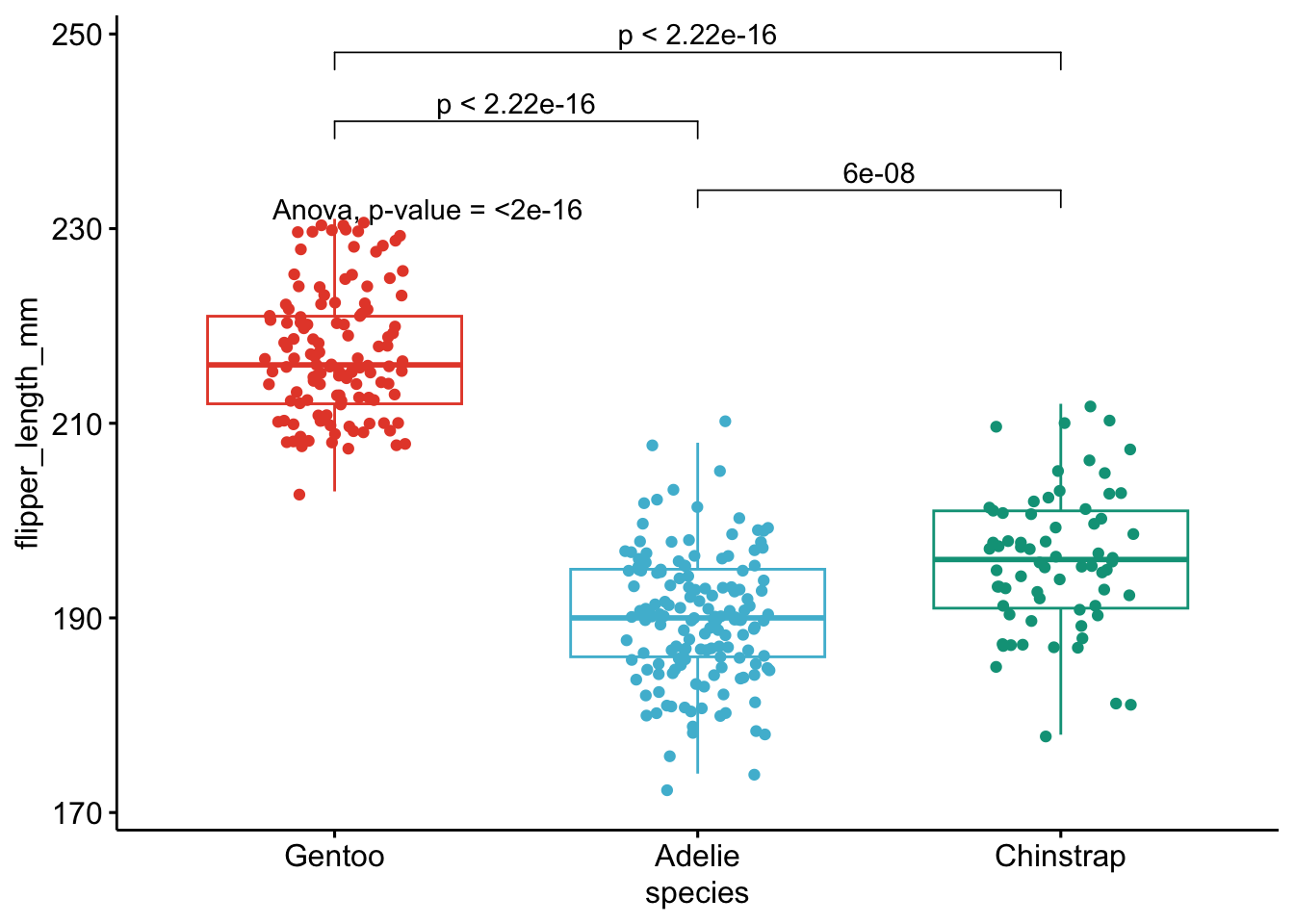
If you are interested in including results of ANOVA and post-hoc tests on the same plot (directly on the boxplots), here are two pieces of code which may be of interest to you.
The first one is edited by me based on the code found in this article:
# Edit from here
x <- which(names(dat) == "species") # name of grouping variable
y <- which(
  names(dat) == "flipper_length_mm" # names of variables to test
)
method1 <- "anova" # one of "anova" or "kruskal.test"
method2 <- "t.test" # one of "wilcox.test" or "t.test"
my_comparisons <- list(c("Chinstrap", "Adelie"), c("Gentoo", "Adelie"), c("Gentoo", "Chinstrap")) # comparisons for post-hoc tests
# Edit until here


# Edit at your own risk
library(ggpubr)
for (i in y) {
  for (j in x) {
    p <- ggboxplot(dat,
      x = colnames(dat[j]), y = colnames(dat[i]),
      color = colnames(dat[j]),
      legend = "none",
      palette = "npg",
      add = "jitter"
    )
    print(
      p + stat_compare_means(aes(label = paste0(after_stat(method), ", p-value = ", after_stat(p.format))),
        method = method1, label.y = max(dat[, i], na.rm = TRUE)
      )
      + stat_compare_means(comparisons = my_comparisons, method = method2, label = "p.format") # remove if p-value of ANOVA or Kruskal-Wallis test >= alpha
    )
  }
}
And the second method is from the {ggstatsplot} package:
library(ggstatsplot)

ggbetweenstats(
  data = dat,
  x = species,
  y = flipper_length_mm,
  type = "parametric", # ANOVA or Kruskal-Wallis
  var.equal = TRUE, # ANOVA or Welch ANOVA
  plot.type = "box",
  pairwise.comparisons = TRUE,
  pairwise.display = "significant",
  centrality.plotting = FALSE,
  bf.message = FALSE
)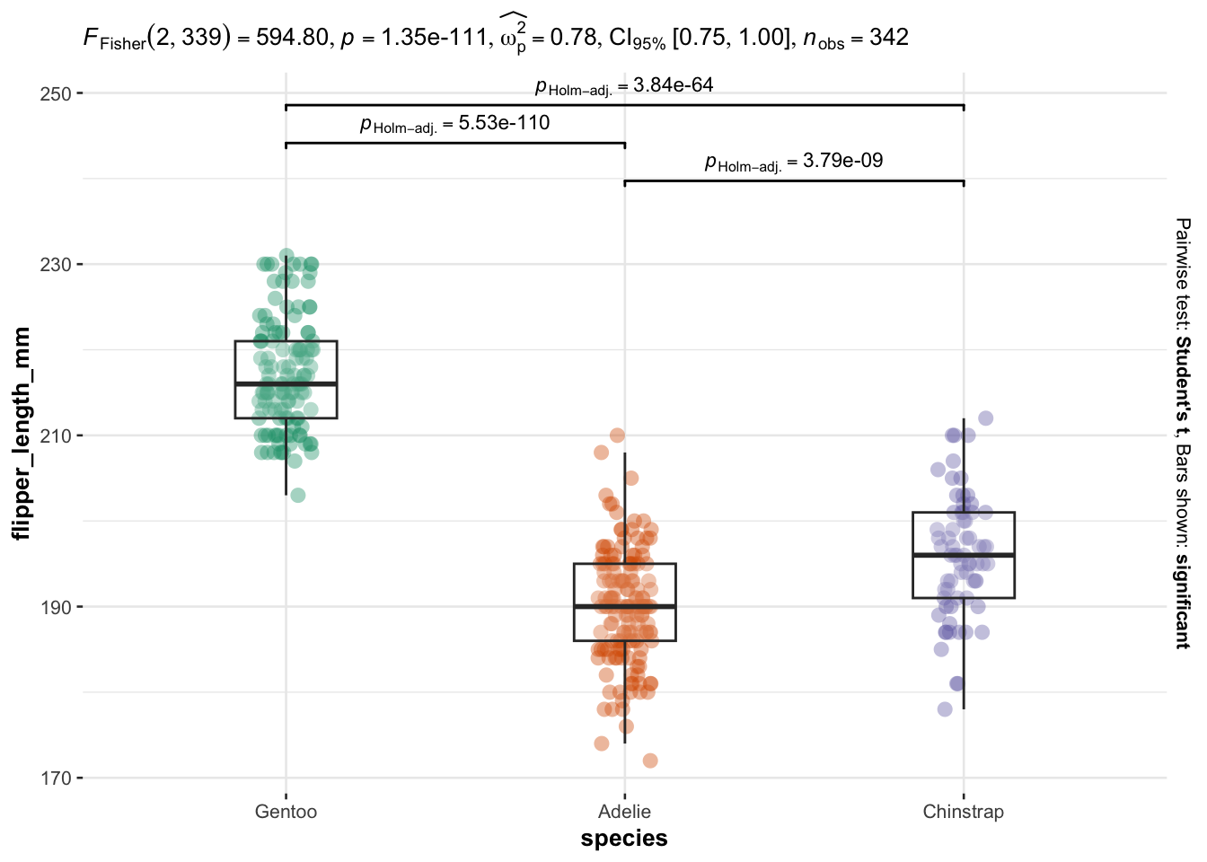
As you can see on the above plot, boxplots by species are presented together with p-values of the ANOVA (after p = in the subtitle of the plot) and p-values of the post-hoc tests (above each comparison).
Besides the fact that these methods can be used to combine a visual representation and statistical results on the same plot, they also have the advantage that you can perform multiple ANOVA tests at once. See more information in this article.
Summary
In this article, we reviewed the goals and hypotheses of an ANOVA, what are the assumptions which need to be verified before being able to trust the results (namely, independence, normality and homogeneity), we then showed how to do an ANOVA in R and how to interpret the results.
An article about ANOVA would not be complete without discussing about post-hoc tests, and in particular, the Tukey HSD—to compare all groups—and the Dunnett’s test—to compare a reference group to all other groups.
Last but not least, we showed how to visualize the data and the results of the ANOVA and post-hoc tests in the same plot.
Thanks for reading. See this tutorial if you would like to learn how to do an ANOVA by hand.
As always, if you have a question or a suggestion related to the topic covered in this article, please add it as a comment so other readers can benefit from the discussion.
(Note that this article is available for download on my Gumroad page.)
References
Note that it is called one-way or one-factor ANOVA because the means relate to the different modalities of a single independent variable, or factor.↩︎
Residuals (denoted \(\epsilon\)) are the differences between the observed values of the dependent variable (\(y\)) and the predicted values (\(\hat{y}\)). In the context of ANOVA, residuals correspond to the differences between the observed values and the mean of all values for that group.↩︎
Stevens (2013) wrote, in p. 57, “Numerous studies have examined the effect of violations of assumptions in ANOVA, and an excellent summary of this literature has been provided by Glass, Peckham, and Sanders (1972). Their review indicates that non normality has only a slight effect on the type I error rate, even for very skewed or kurtotic distributions. For example, the actual \(\alpha\)s for some very non-normal populations were only .055 or .06: very minor deviations from the nominal level of .05. […] The basic reason is the Central Limit Theorem, which states that the sum of independent observations having any distribution whatsoever approaches a normal distribution as the number of observations increases. To be somewhat more specific, Bock (1975) notes,”even for distributions which depart markedly from normality, sums of 50 or more observations approximate to normality. For moderately non-normal distributions the approximation is good with as few as 10 to 20 observations” (p. 111). Now since the sums of independent observations approach normality rapidly, so do the means, and the sampling distribution of F is based on means. Thus the sampling distribution of F is only slightly affected, and therefore the critical values when sampling from normal and non-normal distributions will not differ by much. Lack of normality due to skewness also has only a slight effect on power (a few hundredths).”↩︎
As long as you use the Kruskal-Wallis test to, in fine, compare groups, homoscedasticity is not required. If you wish to compare medians, the Kruskal-Wallis test requires homoscedasticity. See more information about the difference in this article.↩︎
Note that, as discussed in the comments at the end of the article, post-hoc tests can under some circumstances be done directly (without an ANOVA). See the comments or Hsu (1996) for more details.↩︎
Note that you could in principle apply the Bonferroni correction to all tests. For example, in the example above, with 3 tests and a global desired significance level of \(\alpha\) = 0.05, we would only reject a null hypothesis if the p-value is less than \(\frac{0.05}{3}\) = 0.0167. This method is, however, known to be quite conservative, leading to a potentially high rate of false negatives.↩︎
The p-values are adjusted to keep the global significance level to the desired level.↩︎
Thanks Michael Friendly for this suggestion.↩︎
Liked this post?
- Get updates every time a new article is published (no spam and unsubscribe anytime)
- Support the blog
- Share on:


