Step #1: Stating the null and alternative hypothesis

As discussed before, a hypothesis test first requires an idea, that is, an assumption about a phenomenon. This assumption, referred as hypothesis, is derived from the theory and/or the research question.

Since a hypothesis test is used to confirm or refute a prior belief, we need to formulate our belief so that there is a null and an alternative hypothesis. Those hypotheses must be mutually exclusive, which means that they cannot be true at the same time. This is step #1.

In the context of our scenario, the null and alternative hypothesis are thus:

• Null hypothesis \(H_0: \mu = 80\)
• Alternative hypothesis \(H_1: \mu \ne 80\)

When stating the null and alternative hypothesis, bear in mind the following three points:

1. We are always interested in the population and not in the sample. This is the reason \(H_0\) and \(H_1\) will always be written in terms of the population and not in terms of the sample (in this case, \(\mu\) and not \(\bar{x}\)).
2. The assumption we would like to test is often the alternative hypothesis. If the researcher wanted to test whether the mean weight of Belgian adults was less than 80 kg, she would have stated \(H_0: \mu = 80\) (or equivalently, \(H_0: \mu \ge 80\)) and \(H_1: \mu < 80\).⁴ Do not mix the null with the alternative hypothesis, or the conclusions will be diametrically opposed!
3. The null hypothesis is often the status quo. For instance, suppose that a doctor wants to test whether the new treatment A is more efficient than the old treatment B. The status quo is that the new and old treatments are equally efficient. Assuming a larger value is better, she will then write \(H_0: \mu_A = \mu_B\) (or equivalently, \(H_0: \mu_A - \mu_B = 0\)) and \(H_1: \mu_A > \mu_B\) (or equivalently, \(H_0: \mu_A - \mu_B > 0\)). On the opposite, if the lower the better, she would have written \(H_0: \mu_A = \mu_B\) (or equivalently, \(H_0: \mu_A - \mu_B = 0\)) and \(H_1: \mu_A < \mu_B\) (or equivalently, \(H_0: \mu_A - \mu_B < 0\)).

Step #2: Computing the test statistic

The test statistic (often called t-stat) is, in some sense, a metric indicating how extreme the observations are compared to the null hypothesis. The higher the t-stat (in absolute value), the more extreme the observations are.

There are several formulas to compute the t-stat, with one formula for each type of hypothesis test—one or two means, one or two proportions, one or two variances. This means that there is a formula to compute the t-stat for a hypothesis test on one mean, another formula for a test on two means, another for a test on one proportion, etc.⁵

The only difficulty in this second step is to choose the appropriate formula. As soon as you know which formula to use based on the type of test, you simply have to apply it to the data. For the interested reader, see the different formulas to compute the t-stat for the most common tests in this Shiny app.

Luckily, formulas for hypothesis tests on one and two means, and one and two proportions follow the same structure.

Computing the test statistic for these tests is similar than scaling a random variable (a process also knows as “standardization” or “normalization”) which consists in subtracting the mean from that random variable, and dividing the result by the standard deviation:

\[Z = \frac{X - \mu}{\sigma}\]

For these 4 hypothesis tests (one/two means and one/two proportions), computing the test statistic is like scaling the estimator (computed from the sample) corresponding to the parameter of interest (in the population). So we basically subtract the target parameter from the point estimator and then divide the result by the standard error (which is equivalent to the standard deviation but for an estimator).

If this is unclear, here is how the test statistic (denoted \(t_{obs}\)) is computed in our scenario (assuming that the variance of the population is unknown):

\[t_{obs} = \frac{\bar{x} - \mu}{\frac{s}{\sqrt{n}}}\]

where:

• \(\bar{x}\) is the sample mean (i.e., the estimator)
• \(\mu\) is the mean under the null hypothesis (i.e., the target parameter)
• \(s\) is the sample standard deviation
• \(n\) is the sample size
• (\(\frac{s}{\sqrt{n}}\) is the standard error)

Notice the similarity between the formula of this test statistic and the formula used to standardize a random variable. This structure is the same for a test on two means, one proportion and two proportions, except that the estimator, the parameter and the standard error are, of course, slightly different for each type of test.

Suppose that in our case we have a sample mean of 71 kg (\(\bar{x}\) = 71), a sample standard deviation of 13 kg (\(s\) = 13) and a sample size of 10 adults (\(n\) = 10). Remember that the population mean (the mean under the null hypothesis) is 80 kg (\(\mu\) = 80).

The t-stat is thus:

\[t_{obs} = \frac{\bar{x} - \mu}{\frac{s}{\sqrt{n}}} = \frac{71 - 80}{\frac{13}{\sqrt{10}}} = -2.189\]

Although formulas are different depending on which parameter you are testing, the value found for the test statistic gives us an indication on how extreme our observations are.

We keep this value of -2.189 in mind because it will be used again in step #4.

Step #3: Finding the critical value

Although the t-stat gives us an indication of how extreme our observations are, we cannot tell whether this “score of extremity” is too extreme or not based on its value only.

So, at this point, we cannot yet tell whether our data are too extreme or not. For this, we need to compare our t-stat with a threshold—referred as critical value—given by the probability distribution tables (and which can, of course, also be found with R).

In the same way that the formula to compute the t-stat is different for each parameter of interest, the underlying probability distribution—and thus the statistical table—on which the critical value is based is also different for each target parameter. This means that, in addition to choosing the appropriate formula to compute the t-stat, we also need to select the appropriate probability distribution depending on the parameter we are testing.

Luckily, there are only 4 different probability distributions for the 6 hypothesis tests covered in this article (one/two means, one/two proportions and one/two variances):

1. Standard Normal distribution:
   • test on one and two means with known population variance(s)
   • test on two paired samples where the variance of the difference between the 2 samples \(\sigma^2_D\) is known
   • test on one and two proportions (given that some assumptions are met)
2. Student distribution:
   • test on one and two means with unknown population variance(s)
   • test on two paired samples where the variance of the difference between the 2 samples \(\sigma^2_D\) is unknown
3. Chi-square distribution:
   • test on one variance
4. Fisher distribution:
   • test on two variances

Each probability distribution also has its own parameters (up to two parameters for the 4 distribution considered here), defining its shape and/or location. Parameter(s) of a probability distribution can be seen as its DNA; meaning that the distribution is entirely defined by its parameter(s).

Taking our initial scenario—a health professional who would like to test whether the mean weight of Belgian adults is different than 80 kg—as example.

The underlying probability distribution of a test on one mean is either the standard Normal or the Student distribution, depending on whether the variance of the population (not sample variance!) is known or unknown:⁶

• If the population variance is known \(\rightarrow\) the standard Normal distribution is used
• If the population variance is unknown \(\rightarrow\) the Student distribution is used

If no population variance is explicitly given, you can assume that it is unknown since you cannot compute it based on a sample. If you could compute it, that would mean you have access to the entire population and there is, in this case, no point in performing a hypothesis test (you could simply use some descriptive statistics to confirm or refute your belief).

In our example, no population variance is specified so it is assumed to be unknown. We therefore use the Student distribution.

The Student distribution has one parameter which defines it; the number of degrees of freedom. The number of degrees of freedom depends on the type of hypothesis test. For instance, the number of degrees of freedom for a test on one mean is equal to the number of observations minus one (\(n\) - 1). Without going too far into the details, the - 1 comes from the fact that there is one quantity which is estimated (i.e., the mean).⁷ The sample size being equal to 10 in our example, the degrees of freedom is equal to \(n\) - 1 = 10 - 1 = 9.

There is only one last element missing to find the critical value: the significance level. The significance level, denoted \(\alpha\), is the probability of wrongly rejecting the null hypothesis, so the probability of rejecting the null hypothesis although it is in reality true. In this sense, it is an error (type I error, as opposed to the type II error⁸) that we accept to deal with, in order to be able to draw conclusions about a population based on a subset of it.

As you may have read in many statistical textbooks, the significance level is very often set to 5%.⁹ In some fields (such as medicine or engineering, among others), the significance level is also sometimes set to 1% to decrease the error rate.

It is best to specify the significance level before performing a hypothesis test to avoid the temptation to set the significance level in accordance to the results (the temptation is even bigger when the results are on the edge of being significant). As I always tell my students, you cannot “guess” nor compute the significance level. Therefore, if it is not explicitly specified, you can safely assume it is 5%. In our case, we did not indicate it, so we take \(\alpha\) = 5% = 0.05.

Furthermore, in our example, we want to test whether the mean weight of Belgian adults is different than 80 kg. Since we do not specify the direction of the test, it is a two-sided test. If we wanted to test that the mean weight was less than 80 kg (\(H_1: \mu <\) 80) or greater than 80 kg (\(H_1: \mu >\) 80), we would have done a one-sided test.

Make sure that you perform the correct test (two-sided or one-sided) because it has an impact on how to find the critical value (see more in the following paragraphs).

So now that we know the appropriate distribution (Student distribution), its parameter (degrees of freedom (df) = 9), the significance level (\(\alpha\) = 0.05) and the direction (two-sided), we have all we need to find the critical value in the statistical tables:

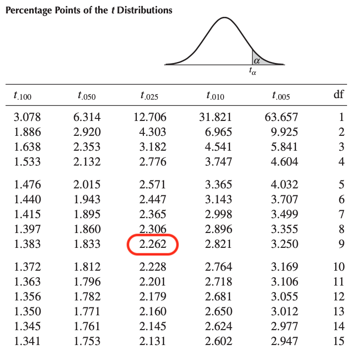
By looking at the row df = 9 and the column \(t_.025\) in the Student’s distribution table, we find a critical value of:

\[t_{n-1; \alpha / 2} = t_{9; 0.025} = 2.262\]

One may wonder why we take \(t_{\alpha/2} = t_.025\) and not \(t_\alpha = t_.05\) since the significance level is 0.05. The reason is that we are doing a two-sided test (\(H_1: \mu \ne\) 80), so the error rate of 0.05 must be divided in 2 to find the critical value to the right of the distribution. Since the Student’s distribution is symmetric, the critical value to the left of the distribution is simply: -2.262.

Visually, the error rate of 0.05 is partitioned into two parts:

• 0.025 to the left of -2.262 and
• 0.025 to the right of 2.262

We keep in mind these critical values of -2.262 and 2.262 for the fourth and last step.

Note that the red shaded areas in the previous plot are also known as the rejection regions. More on that in the following section.

These critical values can also be found in R, thanks to the qt() function:

qt(0.025, df = 9, lower.tail = TRUE)

## [1] -2.262157

qt(0.025, df = 9, lower.tail = FALSE)

## [1] 2.262157

The qt() function is used for the Student’s distribution (q stands for quantile and t for Student). There are other functions accompanying the different distributions:

• qnorm() for the Normal distribution
• qchisq() for the Chi-square distribution
• qf() for the Fisher distribution

Step #4: Concluding and interpreting the results

In this fourth and last step, all we have to do is to compare the test statistic (computed in step #2) with the critical values (found in step #3) in order to conclude the hypothesis test.

The only two possibilities when concluding a hypothesis test are:

1. Rejection of the null hypothesis
2. Non-rejection of the null hypothesis

In our example of adult weight, remember that:

• the t-stat is -2.189
• the critical values are -2.262 and 2.262

Also remember that:

• the t-stat gives an indication on how extreme our sample is compared to the null hypothesis
• the critical values are the threshold from which the t-stat is considered as too extreme

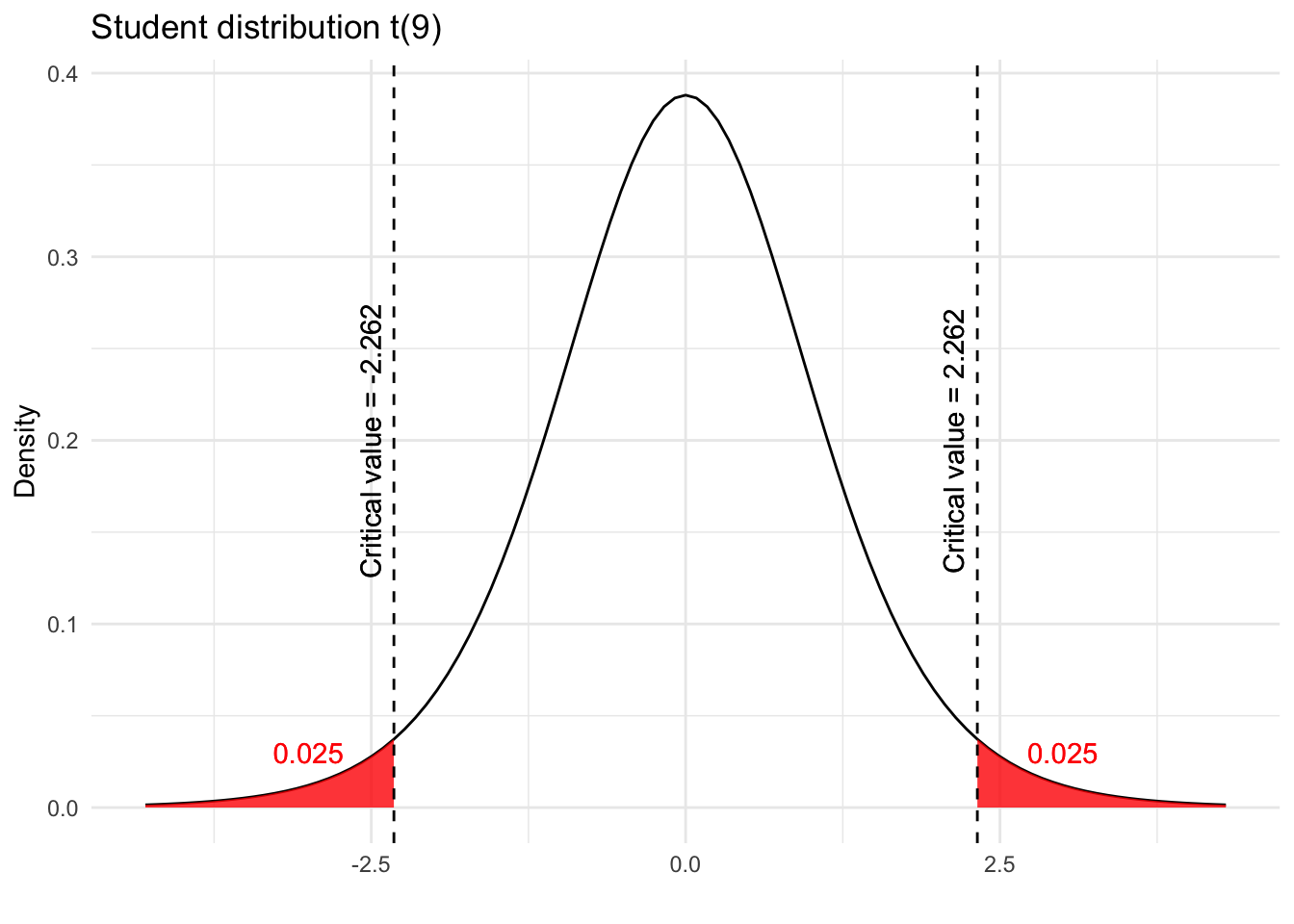
To compare the t-stat with the critical values, I always recommend to plot them:

These two critical values form the rejection regions (the red shaded areas):

• from \(- \infty\) to -2.262, and
• from 2.262 to \(\infty\)

If the t-stat lies within one of the rejection region, we reject the null hypothesis. On the contrary, if the t-stat does not lie within any of the rejection region, we do not reject the null hypothesis.

As we can see from the above plot, the t-stat is less extreme than the critical value and therefore does not lie within any of the rejection region. In conclusion, we do not reject the null hypothesis that \(\mu = 80\).

This is the conclusion in statistical terms but they are meaningless without proper interpretation. So it is a good practice to also interpret the result in the context of the problem:

At the 5% significance level, we do not reject the hypothesis that the mean weight of Belgian adults is 80 kg.

Step #1: Stating the null and alternative hypothesis

The null and alternative hypotheses remain the same:

• \(H_0: \mu = 80\)
• \(H_1: \mu \ne 80\)

Step #2: Computing the test statistic

Remember that the formula for the t-stat is different depending on the type of hypothesis test (one or two means, one or two proportions, one or two variances). In our case of one mean with unknown variance, we have:

\[t_{obs} = \frac{\bar{x} - \mu}{\frac{s}{\sqrt{n}}} = \frac{71 - 80}{\frac{13}{\sqrt{10}}} = -2.189\]

Step #3: Computing the p-value

The p-value is the probability (so it goes from 0 to 1) of observing a sample at least as extreme as the one we observed if the null hypothesis were true. In some sense, it gives you an indication on how likely your null hypothesis is. It is also defined as the smallest level of significance for which the data indicate rejection of the null hypothesis.

For more information about the p-value, I recommend reading this note about the p-value and the significance level \(\alpha\).

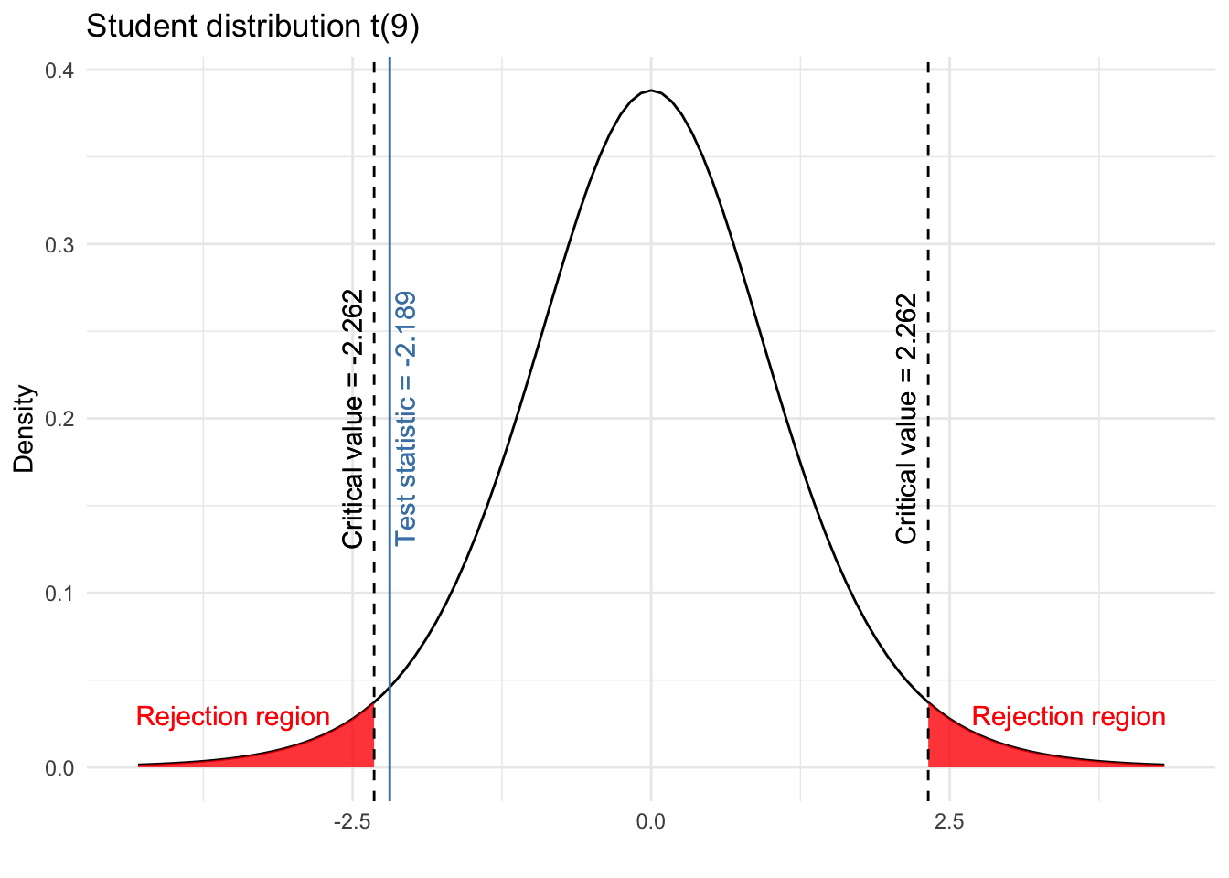
Formally, the p-value is the area beyond the test statistic. Since we are doing a two-sided test, the p-value is thus the sum of the area above 2.189 and below -2.189.

Visually, the p-value is the sum of the two blue shaded areas in the following plot:

The p-value can computed with precision in R with the pt() function:

p_val <- pt(-2.189, df = 9, lower.tail = TRUE) + pt(2.189, df = 9, lower.tail = FALSE)
p_val

## [1] 0.05634202

# which is equivalent than:
p_val <- 2 * pt(2.189, df = 9, lower.tail = FALSE)
p_val

## [1] 0.05634202

The p-value is 0.0563, which indicates that there is a 5.63% chance to observe a sample at least as extreme as the one observed if the null hypothesis were true. This already gives us a hint on whether our t-stat is too extreme or not (and thus whether our null hypothesis is likely or not), but we formally conclude in step #4.

Like the qt() function to find the critical value, we use pt() to find the p-value because the underlying distribution is the Student’s distribution.

Use pnorm(), pchisq() and pf() for the Normal, Chi-square and Fisher distribution, respectively. See also this Shiny app to compute the p-value given a certain t-stat for most probability distributions.

If you do not have access to a computer (during exams for example) you will not be able to compute the p-value precisely, but you can bound it using the statistical table referring to your test.

In our case, we use the Student distribution and we look at the row df = 9 (since df = n - 1):

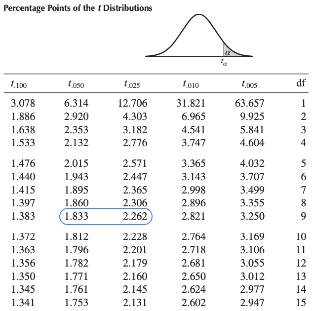
1. The test statistic is -2.189
2. We take the absolute value, which gives 2.189
3. The value 2.189 is between 1.833 and 2.262 (highlighted in blue in the above table)
4. From the column names \(t_{.050}\) and \(t_{.025}\) related to 1.833 and 2.262, we know that:
   • the area to the right of 1.833 is 0.05
   • the area to the right of 2.262 is 0.025
5. So we know that the area to the right of 2.189 must be between 0.025 and 0.05
6. Since the Student distribution is symmetric, we know that the area to the left of -2.189 must also be between 0.025 and 0.05
7. Therefore, the sum of the two areas must be between 0.05 and 0.10
8. In other words, the p-value is between 0.05 and 0.10 (i.e., 0.05 < p-value < 0.10)

Although we could not compute it precisely, it is enough to conclude our hypothesis test in the last step.

Step #4: Concluding and interpreting the results

The final step is now to simply compare the p-value (computed in step #3) with the significance level \(\alpha\). As for all statistical tests:

• If the p-value is smaller than \(\alpha\) (p-value < 0.05) \(\rightarrow H_0\) is unlikely \(\rightarrow\) we reject the null hypothesis
• If the p-value is greater than or equal to \(\alpha\) (p-value \(\ge\) 0.05) \(\rightarrow H_0\) is likely \(\rightarrow\) we do not reject the null hypothesis

No matter if we take into consideration the exact p-value (i.e., 0.0563) or the bounded one (0.05 < p-value < 0.10), it is larger than 0.05, so we do not reject the null hypothesis.¹⁰ In the context of the problem, we do not reject the null hypothesis that the mean weight of Belgian adults is 80 kg.

Remember that rejecting (or not rejecting) a null hypothesis at the significance level \(\alpha\) using the critical value method (method A) is equivalent to rejecting (or not rejecting) the null hypothesis when the p-value is lower (equal or greater) than \(\alpha\) (method B).

This is the reason we find the exact same conclusion than with method A, and why you should too if you use both methods on the same data and with the same significance level.

Step #1: Stating the null and alternative hypothesis

The null and alternative hypotheses remain the same:

• \(H_0: \mu = 80\)
• \(H_1: \mu \ne 80\)

Step #2: Computing the confidence interval

Like hypothesis testing, confidence intervals are a well-known tool in inferential statistics.

Confidence interval is an estimation procedure which produces an interval (i.e., a range of values) containing the true parameter with a certain—usually high—probability.

In the same way that there is a formula for each type of hypothesis test when computing the test statistics, there exists a formula for each type of confidence interval. Formulas for the different types of confidence intervals can be found in this Shiny app.

Here is the formula for a confidence interval on one mean \(\mu\) (with unknown population variance):

\[ (1-\alpha)\text{% CI for } \mu = \bar{x} \pm t_{\alpha/2, n - 1} \frac{s}{\sqrt{n}} \]

where \(t_{\alpha/2, n - 1}\) is found in the Student distribution table (and is similar to the critical value found in step #3 of method A).

Given our data and with \(\alpha\) = 0.05, we have:

\[ \begin{aligned} 95\text{% CI for } \mu &= \bar{x} \pm t_{\alpha/2, n - 1} \frac{s}{\sqrt{n}} \\ &= 71 \pm 2.262 \frac{13}{\sqrt{10}} \\ &= [61.70; 80.30] \end{aligned} \]

The 95% confidence interval for \(\mu\) is [61.70; 80.30] kg. But what does a 95% confidence interval mean?

We know that this estimation procedure has a 95% probability of producing an interval containing the true mean \(\mu\). In other words, if we construct many confidence intervals (with different samples of the same size), 95% of them will, on average, include the mean of the population (the true parameter). So on average, 5% of these confidence intervals will not cover the true mean.

If you wish to decrease this last percentage, you can decrease the significance level (set \(\alpha\) = 0.01 or 0.02 for instance). All else being equal, this will increase the range of the confidence interval and thus increase the probability that it includes the true parameter.

Step #3: Concluding and interpreting the results

The final step is simply to compare the confidence interval (constructed in step #2) with the value of the target parameter (the value under the null hypothesis, mentioned in step #1):

• If the confidence interval does not include the hypothesized value \(\rightarrow H_0\) is unlikely \(\rightarrow\) we reject the null hypothesis
• If the confidence interval includes the hypothesized value \(\rightarrow H_0\) is likely \(\rightarrow\) we do not reject the null hypothesis

In our example:

• the hypothesized value is 80 (since \(H_0: \mu\) = 80)
• 80 is included in the 95% confidence interval since it goes from 61.70 to 80.30 kg
• So we do not reject the null hypothesis

In the terms of the problem, we do not reject the hypothesis that the mean weight of Belgian adults is 80 kg.

As you can see, the conclusion is equivalent than with the critical value method (method A) and the p-value method (method B). Again, this must be the case since we use the same data and the same significance level \(\alpha\) for all three methods.