One-proportion and chi-square goodness of fit test

Antoine Soetewey 2020-05-13 18 minute read

Introduction
In R
By hand
- One-proportion test
  - Verification in R
- Goodness of fit test
  - Verification in R
Conclusion

Introduction

In a previous article, I presented the Chi-square test of independence in R which is used to test the independence between two categorical variables.

In this article, I show how to perform, first in R and then by hand, the:

one-proportion test (also referred as one-sample proportion test)
Chi-square goodness of fit test

The first test is used to compare an observed proportion to an expected proportion, when the qualitative variable has only two categories. The second test is used to compare multiple observed proportions to multiple expected proportions, in a situation where the qualitative variable has two or more categories.

Both tests allow to test the equality of proportions between the levels of the qualitative variable or to test the equality with given proportions. These given proportions could be determined arbitrarily or based on the theoretical probabilities of a known distribution.

In R

Data

For this section, we use the same dataset than in the article on descriptive statistics. It is the well-known iris dataset, to which we add the variable size. The variable size corresponds to small if the length of the petal is smaller than the median of all flowers, big otherwise:

# load iris dataset
dat <- iris

# create size variable
dat$size <- ifelse(dat$Sepal.Length < median(dat$Sepal.Length),
  "small", "big"
)

# show first 5 observations
head(dat, n = 5)

##   Sepal.Length Sepal.Width Petal.Length Petal.Width Species  size
## 1          5.1         3.5          1.4         0.2  setosa small
## 2          4.9         3.0          1.4         0.2  setosa small
## 3          4.7         3.2          1.3         0.2  setosa small
## 4          4.6         3.1          1.5         0.2  setosa small
## 5          5.0         3.6          1.4         0.2  setosa small

One-proportion test

For this example, we have a sample of 150 flowers and we want to test whether the proportion of small flowers is different than the proportion of big flowers (measured by the variable size). Here are the number of flowers by size, and the corresponding proportions:

# barplot
library(ggplot2)
ggplot(dat) +
  aes(x = size) +
  geom_bar(fill = "#0c4c8a") +
  theme_minimal()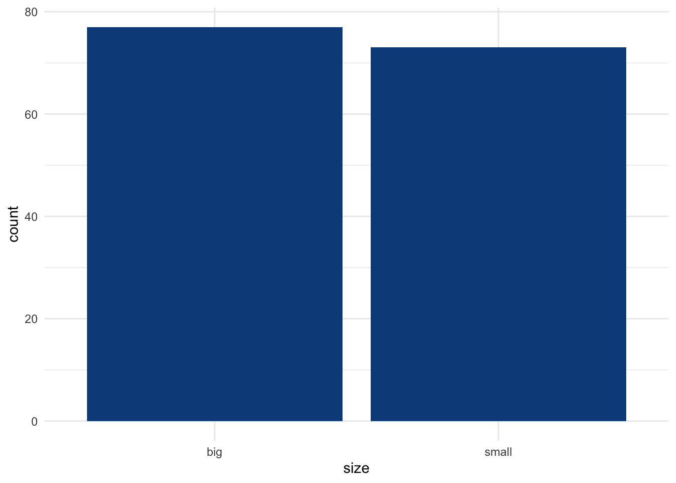

# counts by size
table(dat$size)

## 
##   big small 
##    77    73

# proportions by size, rounded to 2 decimals
round(prop.table(table(dat$size)), 2)

## 
##   big small 
##  0.51  0.49

Among the 150 flowers forming our sample, 51% and 49% are big and small, respectively. To test whether the proportions are different among both sizes, we use the prop.test() function which accepts the following arguments:

number of successes
number of observations/trials
expected probability (the one we want to test against)

The hypotheses in our example are:

$H_0$: proportions of big and small flowers are equal
$H_1$: proportions of big and small flowers are different

Considering (arbitrarily) that big is the success, we have:¹

# one-proportion test
test <- prop.test(
  x = 77, # number of successes
  n = 150, # total number of trials (77 + 73)
  p = 0.5 # we test for equal proportion so prob = 0.5 in each group
)

test

## 
##  1-sample proportions test with continuity correction
## 
## data:  77 out of 150, null probability 0.5
## X-squared = 0.06, df = 1, p-value = 0.8065
## alternative hypothesis: true p is not equal to 0.5
## 95 percent confidence interval:
##  0.4307558 0.5952176
## sample estimates:
##         p 
## 0.5133333

We obtain an output with:

the null probability (0.5),
the test statistic (X-squared = 0.06),
the degrees of freedom (df = 1),
the p-value (p-value = 0.8065),
the alternative hypothesis (true p is not equal to 0.5),
the 95% confidence interval (which can also be extracted with test$conf.int) and
the proportion in the sample (0.5133333).

The p-value is 0.806 so, at the 5% significance level, we do not reject the null hypothesis that the proportions of small and big flowers are the same.

An alternative is the ggpiestats() function from the {ggstatsplot} package:²

## plot with statistical results
library(ggstatsplot)
ggpiestats(
  data = dat,
  x = size,
  bf.message = FALSE
)

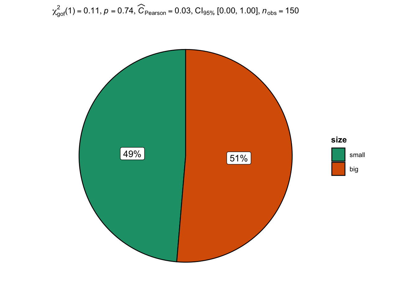
Note that the $p$-value (the value after p = in the subtitle of the plot) is slightly different because Yates’ continuity correction is not applied in ggpiestats() while it is applied by default in prop.test().

The conclusion remains however the same, that is, we do not reject the null hypothesis that proportions of big and small flowers are equal.

Assumption of `prop.test()` and `binom.test()`

Note that prop.test() uses a normal approximation to the binomial distribution. Therefore, one assumption of this test is that the sample size is large enough (usually, n > 30). If the sample size is small, it is recommended to use the exact binomial test.

The exact binomial test can be performed with the binom.test() function and accepts the same arguments as the prop.test() function.

For this example, suppose now that we have a sample of 12 big and 3 small flowers and we want to test whether the proportions are the same among both sizes:

# barplot
barplot(c(12, 3), # observed counts
  names.arg = c("big", "small"), # rename labels
  ylab = "Frequency", # y-axis label
  xlab = "Size" # x-axis label
)
abline(
  h = 15 / 2, # expected counts in each level
  lty = 2 # dashed line
)

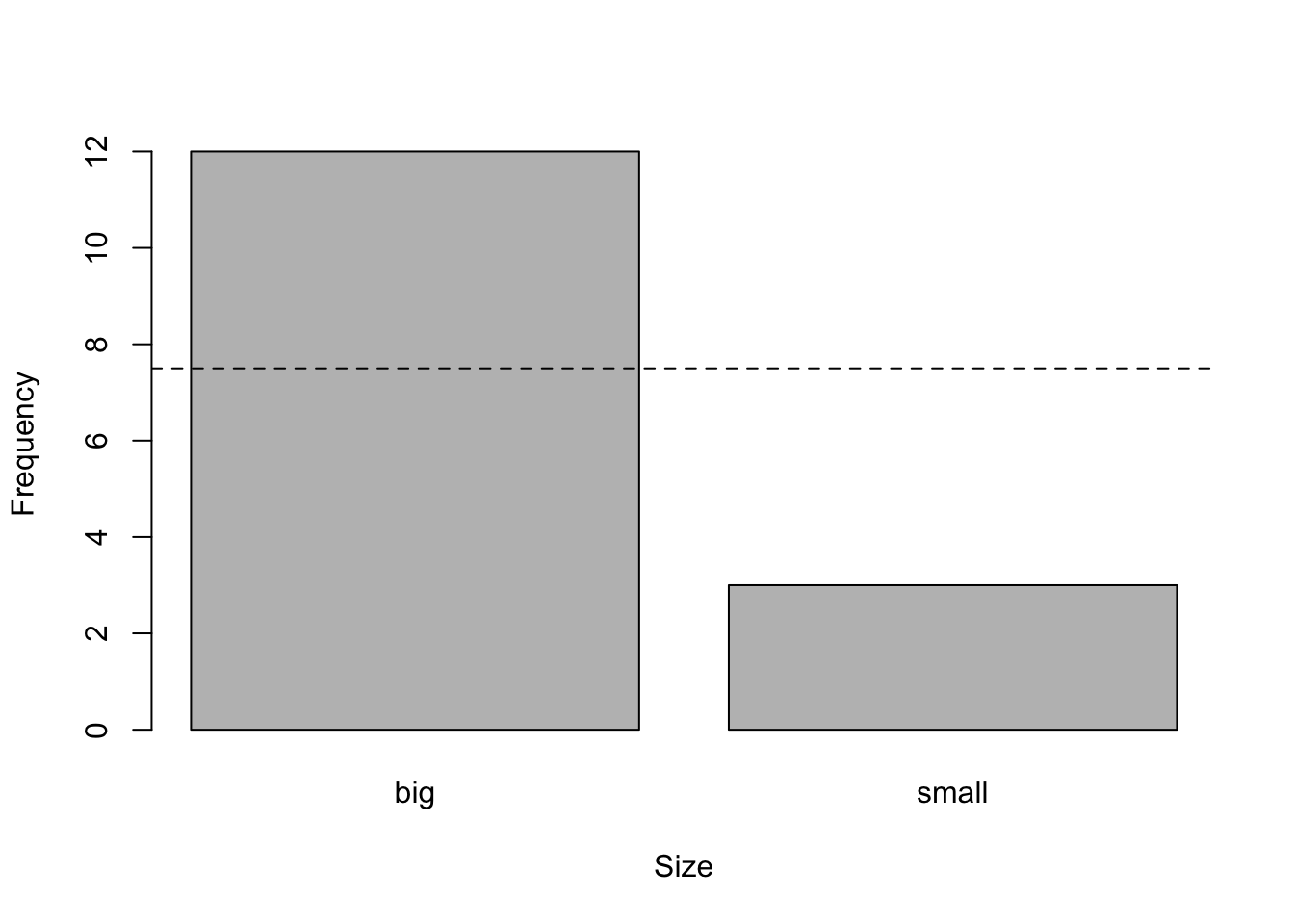
# exact binomial test
test <- binom.test(
  x = 12, # counts of successes
  n = 15, # total counts (12 + 3)
  p = 0.5 # expected proportion
)

test

## 
##  Exact binomial test
## 
## data:  12 and 15
## number of successes = 12, number of trials = 15, p-value = 0.03516
## alternative hypothesis: true probability of success is not equal to 0.5
## 95 percent confidence interval:
##  0.5191089 0.9566880
## sample estimates:
## probability of success 
##                    0.8

The p-value is 0.035 so, at the 5% significance level, we reject the null hypothesis and we conclude that the proportions of small and big flowers are significantly different. This is equivalent than concluding that the proportion of big flowers is significantly different from 0.5 (since there are only two sizes).

If you want to test that the proportion of big flowers is greater than 50%, add the alternative = "greater" argument into the binom.test() function:³

test <- binom.test(
  x = 12, # counts of successes
  n = 15, # total counts (12 + 3)
  p = 0.5, # expected proportion
  alternative = "greater" # test that prop of big flowers is > 0.5
)

test

## 
##  Exact binomial test
## 
## data:  12 and 15
## number of successes = 12, number of trials = 15, p-value = 0.01758
## alternative hypothesis: true probability of success is greater than 0.5
## 95 percent confidence interval:
##  0.5602156 1.0000000
## sample estimates:
## probability of success 
##                    0.8

The p-value is 0.018 so, at the 5% significance level, we reject the null hypothesis and we conclude that the proportion of big flowers is significantly larger than 50%.

Chi-square goodness of fit test

Suppose now that the qualitative variable has more than two levels as it is the case for the variable Species:

# barplot
ggplot(dat) +
  aes(x = Species) +
  geom_bar(fill = "#0c4c8a") +
  theme_minimal()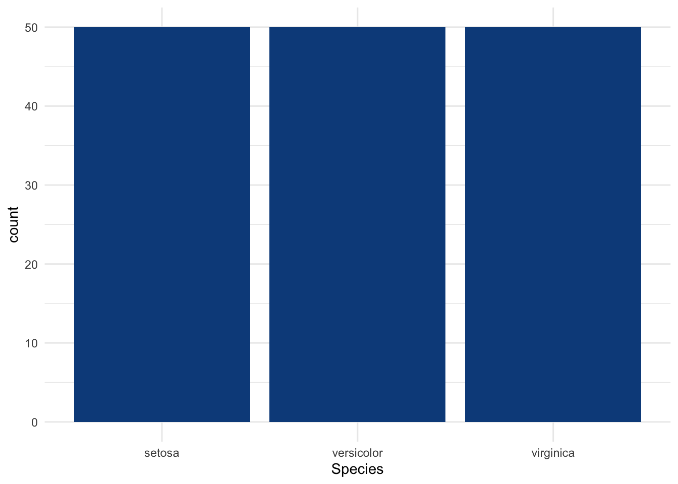

# counts by Species
table(dat$Species)

## 
##     setosa versicolor  virginica 
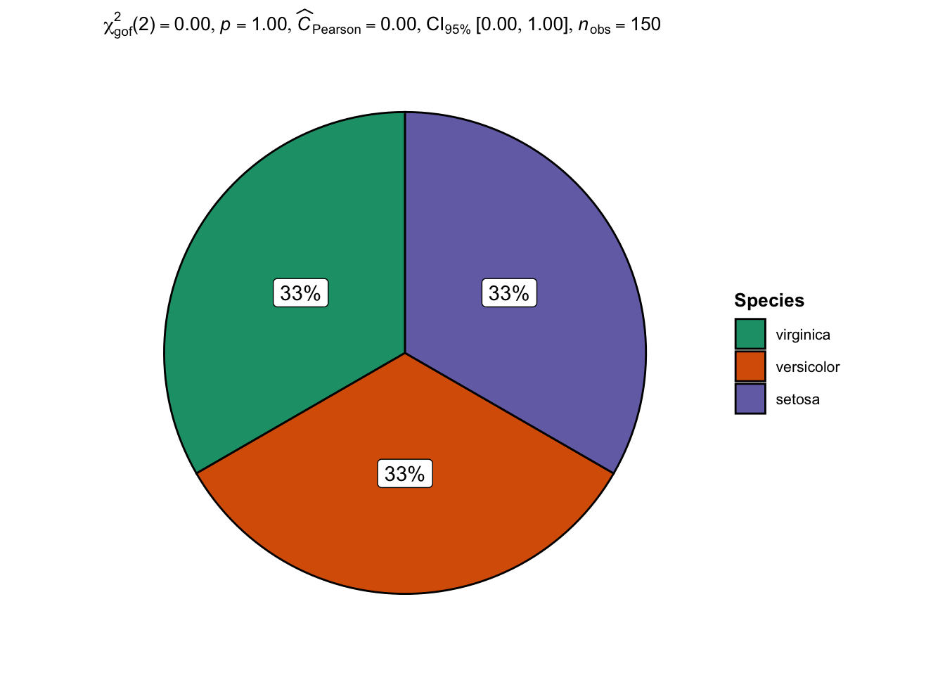
##         50         50         50

The variable Species has 3 levels, with 50 observations in each level.

Suppose for this example that we want to test whether the 3 species are equally common. If they were equally common, they would be equally distributed and the expected proportions would be $\frac{1}{3}$ for each of the species.

The hypotheses are now:

$H_0$: proportions of each species are equal
$H_1$: there is at least one species with a different proportion⁴

This test can be done with the chisq.test() function, accepting the following arguments:

a numeric vector representing the observed proportions
a vector of probabilities (of the same length of the observed proportions) representing the expected proportions

Applied to our research question (i.e., are the 3 species equally common?), we have:

# chi-square goodness of fit test
test <- chisq.test(table(dat$Species), # observed proportions
  p = c(1 / 3, 1 / 3, 1 / 3) # expected proportions
)

test

## 
##  Chi-squared test for given probabilities
## 
## data:  table(dat$Species)
## X-squared = 0, df = 2, p-value = 1

The p-value is 1 so, at the 5% significance level, we do not reject the null hypothesis that the proportions are equal among all species.

This was quite obvious even before doing the statistical test given that there are exactly 50 flowers of each species, so it was easy to see that the species are equally common. We however still did the test to show how it works in practice.

Note that the alternative proposed by the {ggstatsplot} package can also be used for a Chi-square goodness of fit test:

## plot with statistical results
ggpiestats(
  data = dat,
  x = Species,
  bf.message = FALSE
)

Assumptions

One of the assumptions of the chi-square goodness of fit test is that the sample size is large enough in order for the chi-square approximation to be valid.

To be more precise, there must be at least 5 expected frequencies in each group of your categorical variable. This can be verified as follows:

chisq.test(table(dat$Species))$expected

##     setosa versicolor  virginica 
##         50         50         50

The assumption of sufficiently large sample size is met as all expected frequencies are above 5.

Does my distribution follow a given distribution?

In the previous section, we chose the proportions ourselves. The goodness of fit test is also particularly useful to compare observed proportions with expected proportions that are based on some known distribution.

Remember the hypotheses of the test:

$H_0$: there is no significant difference between the observed and the expected frequencies
$H_1$: there is a significant difference between the observed and the expected frequencies

For this example, suppose that we measured the number of girls in 100 families of 5 children. We want to test whether the (observed) distribution of number girls follows a binomial distribution.

Observed frequencies

Here is the distribution of the number of girls per family in our sample of 100 families of 5 children:

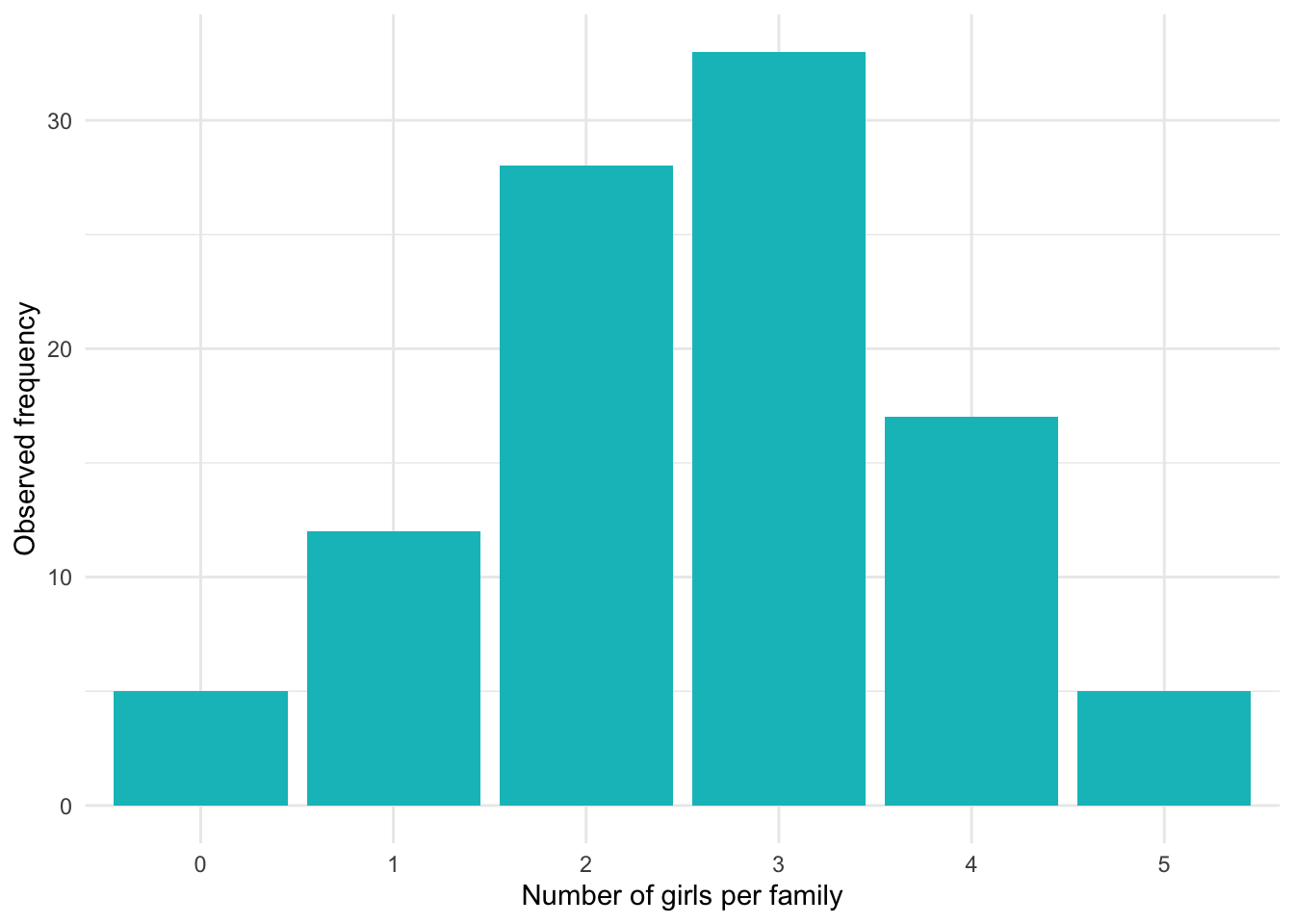
And the corresponding frequencies and relative frequencies (remember that the relative frequency is the frequency divided by the total sample size):

# counts
dat

##   Girls Frequency Relative_freq
## 1     0         5          0.05
## 2     1        12          0.12
## 3     2        28          0.28
## 4     3        33          0.33
## 5     4        17          0.17
## 6     5         5          0.05

Expected frequencies

In order to compare the observed frequencies to a binomial distribution and see if both distributions match, we first need to determine the expected frequencies that would be obtained in case of a binomial distribution.

The expected frequencies assuming a probability of 0.5 of having a girl (for each of the 5 children) are as follows:

# create expected frequencies for a binomial distribution
x <- 0:5
df <- data.frame(
  Girls = factor(x),
  Expected_relative_freq = dbinom(x, size = 5, prob = 0.5)
)
df$Expected_freq <- df$Expected_relative_freq * 100 # *100 since there are 100 families

# create barplot
p <- ggplot(df, aes(x = Girls, y = Expected_freq)) +
  geom_bar(stat = "identity", fill = "#F8766D") +
  xlab("Number of girls per family") +
  ylab("Expected frequency") +
  labs(title = "Binomial distribution Bi(x, n = 5, p = 0.5)") +
  theme_minimal()
p

# expected relative frequencies and (absolute) frequencies
df

##   Girls Expected_relative_freq Expected_freq
## 1     0                0.03125         3.125
## 2     1                0.15625        15.625
## 3     2                0.31250        31.250
## 4     3                0.31250        31.250
## 5     4                0.15625        15.625
## 6     5                0.03125         3.125

Observed vs. expected frequencies

We now compare the observed frequencies to the expected frequencies to see whether the two differ significantly. If the two differ significantly, we reject the hypothesis that the number of girls per family of 5 children follows a binomial distribution. On the other hand, if the observed and expected frequencies are similar, we do not reject the hypothesis that the number of girls per family follows a binomial distribution.

Visually we have:

# create data
data <- data.frame(
  num_girls = factor(rep(c(0:5), times = 2)),
  Freq = c(dat$Freq, df$Expected_freq),
  obs_exp = c(rep("observed", 6), rep("expected", 6))
)

# create plot
ggplot() +
  geom_bar(
    data = data, aes(
      x = num_girls, y = Freq,
      fill = obs_exp
    ),
    position = "dodge", # bar next to each other
    stat = "identity"
  ) +
  ylab("Frequency") +
  xlab("Number of girls per family") +
  theme_minimal() +
  theme(legend.title = element_blank()) # remove legend title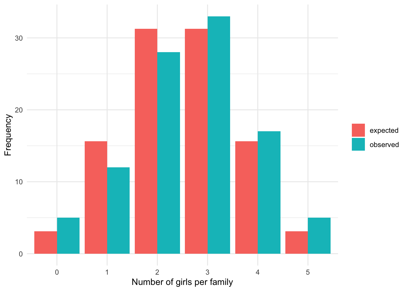

We see that the observed and expected frequencies are quite similar, so we expect that the number of girls in families of 5 children follows a binomial distribution. However, only the goodness of fit test will confirm our belief:

# chi-square goodness of fit test
test <- chisq.test(dat$Freq, # observed frequencies
  p = df$Expected_relative_freq # expected proportions
)

test

## 
##  Chi-squared test for given probabilities
## 
## data:  dat$Freq
## X-squared = 3.648, df = 5, p-value = 0.6011

The p-value is 0.601 so, at the 5% significance level, we do not reject the null hypothesis that the observed and expected frequencies are equal. This is equivalent than concluding that we cannot reject the hypothesis that the number of girls in families of 5 children follows a binomial distribution (since the expected frequencies were based on a binomial distribution).

Note that the chi-square goodness of fit test can of course be performed with other types of distribution than the binomial one. For instance, if you want to test whether an observed distribution follows a Poisson distribution, this test can be used to compare the observed frequencies with the expected proportions that would be obtained in case of a Poisson distribution.

By hand

Now that we showed how to perform the one-proportion and chi-square goodness of fit test in R, in this section we show how to do these tests by hand. We first illustrate the one-proportion test then the chi-square goodness of fit test.

One-proportion test

For this example, suppose that we tossed a coin 100 times and noted that it landed on heads 67 times. Following this, we want to test whether the coin is fair, that is, test whether the probability of landing on heads or tails is equal to 50%.

As for many hypothesis tests, we do it through 4 easy steps:

State the null and alternative hypotheses
Compute the test-statistic (also known as t-stat)
Find the rejection region
Conclude by comparing the test-statistic with the rejection region

Step 1.

In our example, the null and alternative hypotheses are:

$H_0$: $p_0 = 0.5$
$H_1$: $p_0 \ne 0.5$

where $p_0$ is the expected proportion of landing on heads.

Step 2.

The test statistic is:⁵

\[z_{obs} = \frac{\hat{p} - p_0}{\sqrt{\frac{p_0(1 - p_0)}{n}}} = \frac{0.67 - 0.5}{\sqrt{\frac{0.5 \cdot (1 - 0.5)}{100}}} = 3.4\]

(See how to perform hypothesis tests in a Shiny app if you need more help in computing the test statistic.)

Step 3.

The rejection region is found via the normal distribution table. Assuming a significance level $\alpha = 0.05$, we have:

\[\pm z_{\alpha/2} = \pm z_{0.025} = \pm 1.96\]

Step 4.

We compare the test statistic (found in step 2) with the rejection region (found in step 3) and we conclude. Visually, we have:

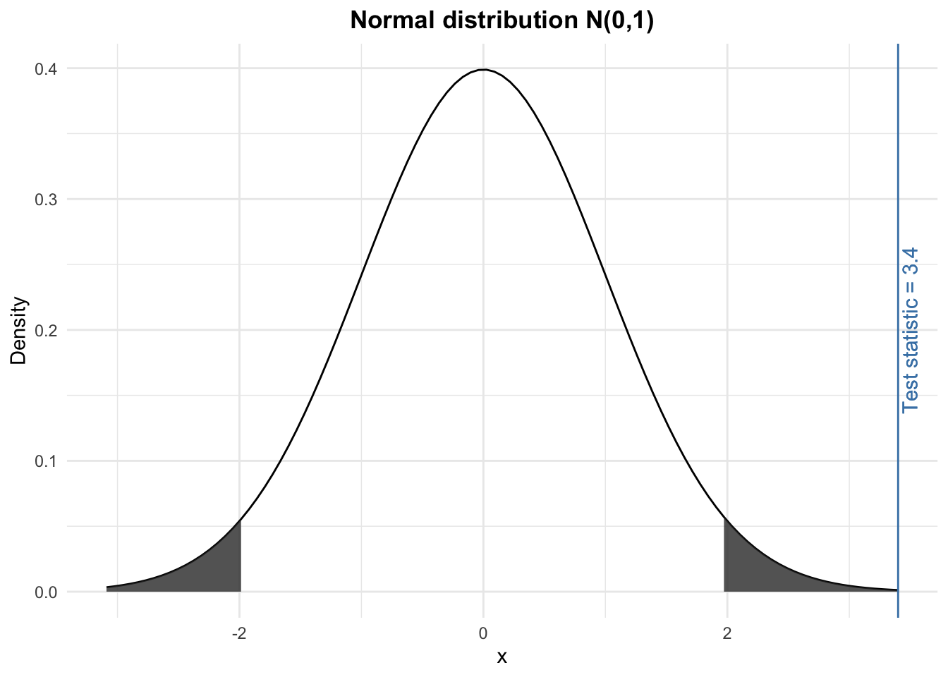
The test statistic lies within the rejection region (i.e., the grey shaded areas). Therefore, at the 5% significance level, we reject the null hypothesis and we conclude that the proportion of heads (and thus tails) is significantly different than 50%. In other words, still at the 5% significance level, we conclude that the coin is unfair.

If you prefer to compute the p-value instead of comparing the t-stat and the rejection region, you can use this Shiny app to easily compute p-values for different probability distributions. After having opened the app, set the t-stat, the corresponding alternative and you will find the p-value at the top of the page.

Verification in R

Just for the sake of illustration, here is the verification of the above example in R:

# one-proportion test
test <- prop.test(
  x = 67, # number of heads
  n = 100, # number of trials
  p = 0.5 # expected probability of heads
)

test

## 
##  1-sample proportions test with continuity correction
## 
## data:  67 out of 100, null probability 0.5
## X-squared = 10.89, df = 1, p-value = 0.0009668
## alternative hypothesis: true p is not equal to 0.5
## 95 percent confidence interval:
##  0.5679099 0.7588442
## sample estimates:
##    p 
## 0.67

The p-value is 0.001 so, at the 5% significance level, we reject the null hypothesis that the proportions of heads and tails are equal, and we conclude that the coin is biased. This is the same conclusion than the one found by hand.

Goodness of fit test

We now illustrate the chi-square goodness of fit test by hand with the following example.

Suppose that we toss a dice 100 times, we note how many times it lands on each face (1 to 6) and we test whether the dice is fair. Here are the observed counts by dice face:

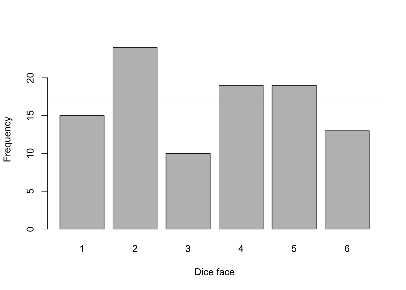
## dice_face
##  1  2  3  4  5  6 
## 15 24 10 19 19 13

With a fair dice, we would expect it to land $\frac{100}{6} \approx 16.67$ times on each face (this expected value is represented by the dashed line in the above plot). Although the observed frequencies are different than the expected value of 16.67:

##   dice_face observed_freq expected_freq
## 1         1            15         16.67
## 2         2            24         16.67
## 3         3            10         16.67
## 4         4            19         16.67
## 5         5            19         16.67
## 6         6            13         16.67

we need to test whether they are significantly different. For this, we perform the appropriate hypothesis test following the 4 easy steps mentioned above:

State the null and alternative hypotheses
Compute the test-statistic (also known as t-stat)
Find the rejection region
Conclude by comparing the test-statistic with the rejection region

Step 1.

The null and alternative hypotheses of the chi-square goodness of fit test are:

$H_0$: there is no significant difference between the observed and the expected frequencies
$H_1$: there is a significant difference between the observed and the expected frequencies

Applied to our example, we have:

$H_0$: all faces occur in the same proportion
$H_1$: at least one proportion is not equal to 1/6

Step 2.

The test statistic is:

\[\chi^2 = \sum_{i = 1}^k \frac{(O_i - E_i)^2}{E_i}\]

where $O_i$ is the observed frequency, $E_i$ is the expected frequency and $k$ is the number of categories (in our case, there are 6 categories, representing the 6 dice faces).

This $\chi^2$ statistic is obtained by calculating the difference between the observed number of cases and the expected number of cases in each category. This difference is squared (to avoid negative and positive differences being compensated) and divided by the expected number of cases in that category. These values are then summed for all categories, and the total is referred to as the $\chi^2$ statistic. Large values of this test statistic lead to the rejection of the null hypothesis, small values mean that the null hypothesis cannot be rejected.⁶

Given our data, we have:

\[\chi^2 = \frac{(15 - 16.67)^2}{16.67} + \frac{(24 - 16.67)^2}{16.67} + \\ \frac{(10 - 16.67)^2}{16.67} +\frac{(19 - 16.67)^2}{16.67} + \\ \frac{(19 - 16.67)^2}{16.67} + \frac{(13 - 16.67)^2}{16.67} = 7.52\]

Step 3.

Whether the $\chi^2$ test statistic is small or large depends on the rejection region. The rejection region is found via the $\chi^2$ distribution table. With a degrees of freedom equals to $k - 1$ (where $k$ is the number of categories) and assuming a significance level $\alpha = 0.05$, we have:

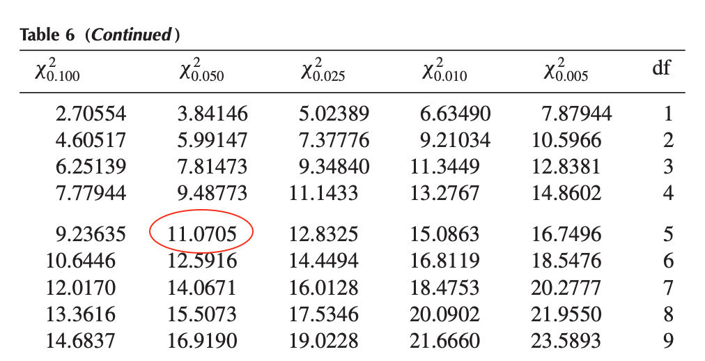
\[\chi^2_{\alpha; k-1} = \chi^2_{0.05; 5} = 11.0705\]

Step 4.

We compare the test statistic (found in step 2) with the rejection region (found in step 3) and we conclude. Visually, we have:

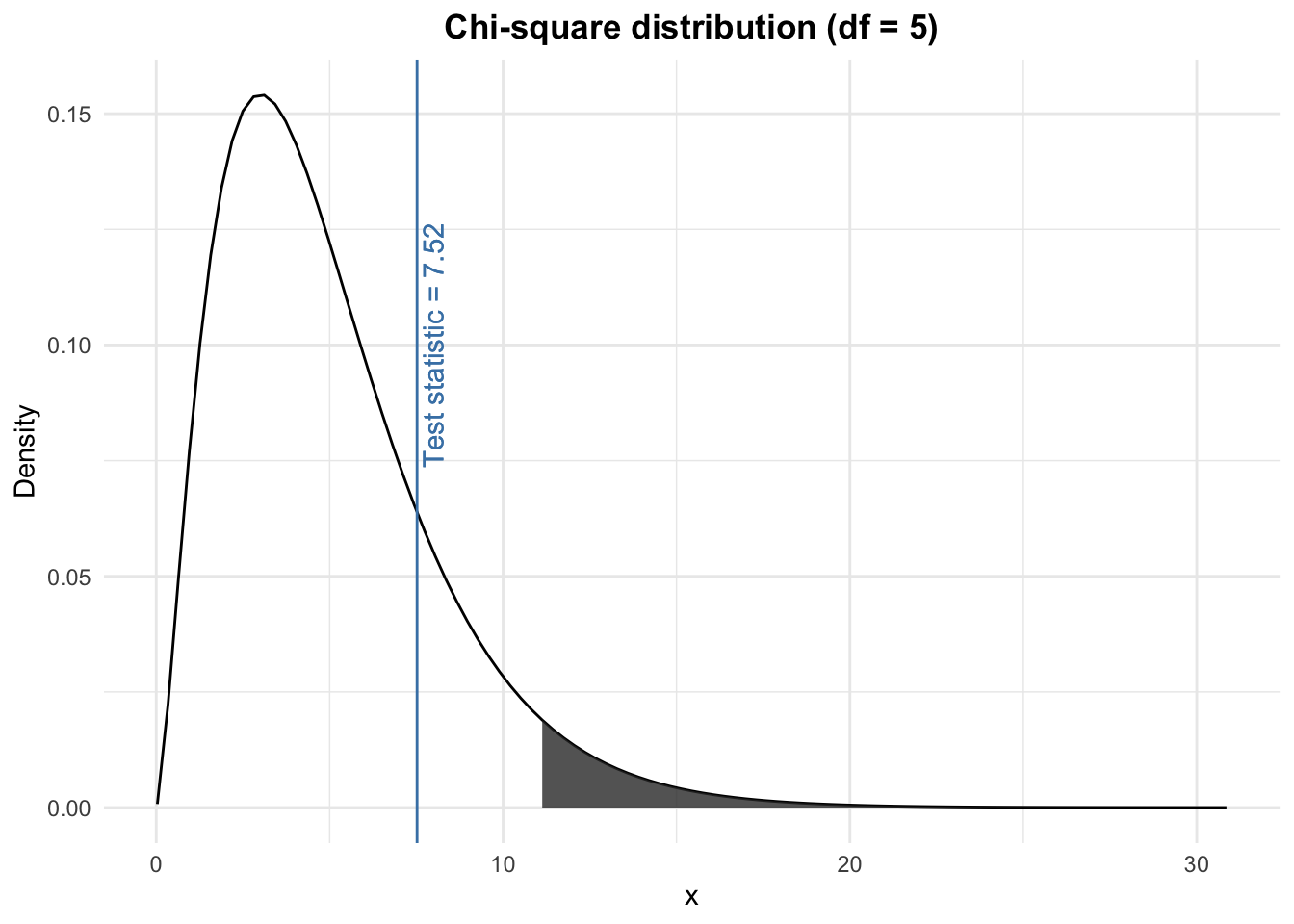
The test statistic does not lie within the rejection region (i.e., the grey shaded area). Therefore, at the 5% significance level, we do not reject the null hypothesis that there is no significant difference between the observed and the expected frequencies. In other words, still at the 5% significance level, we cannot reject the hypothesis that the dice is fair.

Again, you can use the Shiny app to easily compute the p-value given the test statistic if you prefer this method over the comparison between the t-stat and the rejection region.

Verification in R

Just for the sake of illustration, here is the verification of the above example in R:

# chi-square goodness of fit test
test <- chisq.test(dat$observed_freq, # observed frequencies for each dice face
  p = rep(1 / 6, 6) # expected probabilities for each dice face
)

test

## 
##  Chi-squared test for given probabilities
## 
## data:  dat$observed_freq
## X-squared = 7.52, df = 5, p-value = 0.1847

The test statistic and degrees of freedom are exactly the same than the ones found by hand. The p-value is 0.185 which, still at the 5% significance level, leads to the same conclusion than by hand (i.e., failing to reject the null hypothesis).

Conclusion

Thanks for reading.

I hope this article helped you to understand and perform the one-proportion and chi-square goodness of fit test in R and by hand. Learn more about the Chi-square test of independence in R and by hand if you want to analyze two categorical variables instead of one.

As always, if you have a question or a suggestion related to the topic covered in this article, please add it as a comment so other readers can benefit from the discussion.

Choosing big or small as the success event gives the exact same conclusion.↩︎
Note that if possible, it is best to avoid pie charts and use bar charts instead. Unfortunately, the ggbarstats() function works only for the independence Chi-square test.↩︎
Similarly, this argument can also be added to the prop.test() function to test whether the observed proportion is larger than the expected proportion. Use alternative = "less" if you want to test whether the observed proportion is smaller than the expected one.↩︎
Be careful that the alternative hypothesis is not that all proportions are different. One different from the others is sufficient to reject the null hypothesis. It is, in some sense, similar to the alternative hypothesis of the ANOVA which says that at least one mean is different than another.↩︎
One assumption of this test is that $n \cdot p \ge 5$ and $n \cdot (1 - p) \ge 5$. The assumption is met so we can use the normal approximation to the binomial distribution.↩︎
Source: http://uregina.ca/~gingrich/ch10.pdf.↩︎

Liked this post?

Get updates every time a new article is published (no spam and unsubscribe anytime):

Support the blog
Share on:

Stats and R

One-proportion and chi-square goodness of fit test

Introduction

In R

Data

One-proportion test

Assumption of prop.test() and binom.test()

Chi-square goodness of fit test

Assumptions

Does my distribution follow a given distribution?

Observed frequencies

Expected frequencies

Observed vs. expected frequencies

By hand

One-proportion test

Verification in R

Goodness of fit test

Verification in R

Conclusion

Related articles

Liked this post?

Assumption of `prop.test()` and `binom.test()`