
Chi-square test of independence by hand

Introduction
Chi-square tests of independence test whether two qualitative variables are independent, that is, whether there exists a relationship between two categorical variables. In other words, this test is used to determine whether the values of one of the 2 qualitative variables depend on the values of the other qualitative variable.
If the test shows no association between the two variables (i.e., the variables are independent), it means that knowing the value of one variable gives no information about the value of the other variable. On the contrary, if the test shows a relationship between the variables (i.e., the variables are dependent), it means that knowing the value of one variable provides information about the value of the other variable.
This article focuses on how to perform a Chi-square test of independence by hand and how to interpret the results with a concrete example. To learn how to do this test in R, read the article “Chi-square test of independence in R”.
Hypotheses
The Chi-square test of independence is a hypothesis test so it has a null (\(H_0\)) and an alternative hypothesis (\(H_1\)):
- \(H_0\) : the variables are independent, there is no relationship between the two categorical variables. Knowing the value of one variable does not help to predict the value of the other variable
- \(H_1\) : the variables are dependent, there is a relationship between the two categorical variables. Knowing the value of one variable helps to predict the value of the other variable
How the test works?
The Chi-square test of independence works by comparing the observed frequencies (so the frequencies observed in your sample) to the expected frequencies if there was no relationship between the two categorical variables (so the expected frequencies if the null hypothesis was true).
If the difference between the observed frequencies and the expected frequencies is small, we cannot reject the null hypothesis of independence and thus we cannot reject the fact that the two variables are not related. On the other hand, if the difference between the observed frequencies and the expected frequencies is large, we can reject the null hypothesis of independence and thus we can conclude that the two variables are related.
The threshold between a small and large difference is a value that comes from the Chi-square distribution (hence the name of the test). This value, referred as the critical value, depends on the significance level \(\alpha\) (usually set equal to 5%) and on the degrees of freedom. This critical value can be found in the statistical table of the Chi-square distribution. More on this critical value and the degrees of freedom later in the article.
Example
For our example, we want to determine whether there is a statistically significant association between smoking and being a professional athlete. Smoking can only be “yes” or “no” and being a professional athlete can only be “yes” or “no”. The two variables of interest are qualitative variables so we need to use a Chi-square test of independence, and the data have been collected on 28 persons.
Note that we chose binary variables (binary variables = qualitative variables with two levels) for the sake of easiness, but the Chi-square test of independence can also be performed on qualitative variables with more than two levels. For instance, if the variable smoking had three levels: (i) non-smokers, (ii) moderate smokers and (iii) heavy smokers, the steps and the interpretation of the results of the test are similar than with two levels.
Observed frequencies
Our data are summarized in the contingency table below reporting the number of people in each subgroup, totals by row, by column and the grand total:
| Non-smoker | Smoker | Total | |
|---|---|---|---|
| Athlete | 14 | 4 | 18 |
| Non-athlete | 0 | 10 | 10 |
| Total | 14 | 14 | 28 |
Expected frequencies
Remember that for the Chi-square test of independence we need to determine whether the observed counts are significantly different from the counts that we would expect if there was no association between the two variables. We have the observed counts (see the table above), so we now need to compute the expected counts in the case the variables were independent. These expected frequencies are computed for each subgroup one by one with the following formula:
\[\text{exp. frequencies} = \frac{\text{total # of obs. for the row} \cdot \text{total # of obs. for the column}}{\text{total number of observations}}\]
where obs. correspond to observations. Given our table of observed frequencies above, below is the table of the expected frequencies computed for each subgroup:
| Non-smoker | Smoker | Total | |
|---|---|---|---|
| Athlete | (18 * 14) / 28 = 9 | (18 * 14) / 28 = 9 | 18 |
| Non-athlete | (10 * 14) / 28 = 5 | (10 * 14) / 28 = 5 | 10 |
| Total | 14 | 14 | 28 |
Note that the Chi-square test of independence should only be done when the expected frequencies in all groups are equal to or greater than 5. This assumption is met for our example as the minimum number of expected frequencies is 5. If the condition is not met, the Fisher’s exact test is preferred.
Talking about assumptions, the Chi-square test of independence requires that the observations are independent. This is usually not tested formally, but rather verified based on the design of the experiment and on the good control of experimental conditions. If you are not sure, ask yourself if one observation is related to another (if one observation has an impact on another). If not, it is most likely that you have independent observations.
If you have dependent observations (paired samples), the McNemar’s or Cochran’s Q tests should be used instead. The McNemar’s test is used when we want to know if there is a significant change in two paired samples (typically in a study with a measure before and after on the same subject) when the variables have only two categories. The Cochran’s Q tests is an extension of the McNemar’s test when we have more than two related measures.
Test statistic
We have the observed and expected frequencies. We now need to compare these frequencies to determine if they differ significantly. The difference between the observed and expected frequencies, referred as the test statistic (or t-stat) and denoted \(\chi^2\), is computed as follows:
\[\chi^2 = \sum_{i, j} \frac{\big(O_{ij} - E_{ij}\big)^2}{E_{ij}}\]
where \(O\) represents the observed frequencies and \(E\) the expected frequencies. We use the square of the differences between the observed and expected frequencies to make sure that negative differences are not compensated by positive differences. The formula looks more complex than what it really is, so let’s illustrate it with our example. We first compute the difference in each subgroup one by one according to the formula:
- in the subgroup of athlete and non-smoker: \(\frac{(14 - 9)^2}{9} = 2.78\)
- in the subgroup of non-athlete and non-smoker: \(\frac{(0 - 5)^2}{5} = 5\)
- in the subgroup of athlete and smoker: \(\frac{(4 - 9)^2}{9} = 2.78\)
- in the subgroup of non-athlete and smoker: \(\frac{(10 - 5)^2}{5} = 5\)
and then we sum them all to obtain the test statistic:
\[\chi^2 = 2.78 + 5 + 2.78 + 5 = 15.56\]
Critical value
The test statistic alone is not enough to conclude for independence or dependence between the two variables. As previously mentioned, this test statistic (which in some sense is the difference between the observed and expected frequencies) must be compared to a critical value to determine whether the difference is large or small. One cannot tell that a test statistic is large or small without putting it in perspective with the critical value.
If the test statistic is above the critical value, it means that the probability of observing such a difference between the observed and expected frequencies is unlikely. On the other hand, if the test statistic is below the critical value, it means that the probability of observing such a difference is likely. If it is likely to observe this difference, we cannot reject the hypothesis that the two variables are independent, otherwise we can conclude that there exists a relationship between the variables.
The critical value can be found in the statistical table of the Chi-square distribution and depends on the significance level, denoted \(\alpha\), and the degrees of freedom, denoted \(df\). The significance level is usually set equal to 5%. The degrees of freedom for a Chi-square test of independence is found as follow:
\[df = (\text{number of rows} - 1) \cdot (\text{number of columns} - 1)\]
In our example, the degrees of freedom is thus \(df = (2 - 1) \cdot (2 - 1) = 1\) since there are two rows and two columns in the contingency table (totals do not count as a row or column).
We now have all the necessary information to find the critical value in the Chi-square table (\(\alpha = 0.05\) and \(df = 1\)). To find the critical value we need to look at the row \(df = 1\) and the column \(\chi^2_{0.050}\) (since \(\alpha = 0.05\)) in the picture below. The critical value is \(3.84146\).1
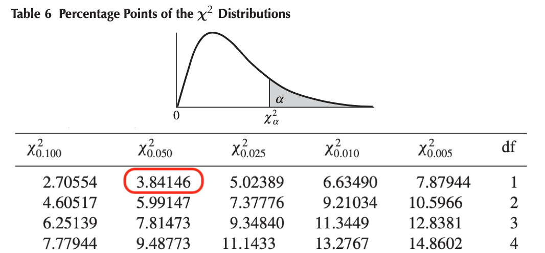
Chi-square table - Critical value for alpha = 5% and df = 1
Conclusion and interpretation
Now that we have the test statistic and the critical value, we can compare them to check whether the null hypothesis of independence of the variables is rejected or not. In our example,
\[\text{test statistic} = 15.56 > \text{critical value} = 3.84146\]
Like for many statistical tests, when the test statistic is larger than the critical value, we can reject the null hypothesis at the specified significance level.
In our case, we can therefore reject the null hypothesis of independence between the two categorical variables at the 5% significance level.
\(\Rightarrow\) This means that there is a significant relationship between the smoking habit and being an athlete or not. Knowing the value of one variable helps to predict the value of the other variable.
Thanks for reading.
I hope the article helped you to perform the Chi-square test of independence by hand and interpret its results. If you would like to learn how to do this test in R, read the article “Chi-square test of independence in R”.
As always, if you have a question or a suggestion related to the topic covered in this article, please add it as a comment so other readers can benefit from the discussion.
Liked this post?
- Get updates every time a new article is published (no spam and unsubscribe anytime)
- Support the blog
- Share on:


