
Fisher's exact test in R: independence test for a small sample

Introduction
After presenting the Chi-square test of independence by hand and in R, this article focuses on the Fisher’s exact test.
Independence tests are used to determine if there is a significant relationship between two categorical variables. There exists two different types of independence test:
- the Chi-square test (the most common)
- the Fisher’s exact test
On the one hand, the Chi-square test is used when the sample is large enough (in this case the \(p\)-value is an approximation that becomes exact when the sample becomes infinite, which is the case for many statistical tests). On the other hand, the Fisher’s exact test is used when the sample is small (and in this case the \(p\)-value is exact and is not an approximation).
The literature indicates that the usual rule for deciding whether the \(\chi^2\) approximation is good enough is that the Chi-square test is not appropriate when the expected values in one of the cells of the contingency table is less than 5, and in this case the Fisher’s exact test is preferred (McCrum-Gardner 2008; Bower 2003).
Hypotheses
The hypotheses of the Fisher’s exact test are the same than for the Chi-square test, that is:
- \(H_0\) : the variables are independent, there is no relationship between the two categorical variables. Knowing the value of one variable does not help to predict the value of the other variable
- \(H_1\) : the variables are dependent, there is a relationship between the two categorical variables. Knowing the value of one variable helps to predict the value of the other variable
Example
Data
For our example, we want to determine whether there is a statistically significant association between smoking and being a professional athlete. Smoking can only be “yes” or “no” and being a professional athlete can only be “yes” or “no”. The two variables of interest are qualitative variables and we collected data on 14 persons.1
Observed frequencies
Our data are summarized in the contingency table below reporting the number of people in each subgroup:
dat <- data.frame(
  "smoke_no" = c(7, 0),
  "smoke_yes" = c(2, 5),
  row.names = c("Athlete", "Non-athlete"),
  stringsAsFactors = FALSE
)
colnames(dat) <- c("Non-smoker", "Smoker")

dat
## Non-smoker Smoker
## Athlete 7 2
## Non-athlete 0 5It is also a good practice to draw a mosaic plot to visually represent the data:
mosaicplot(dat,
  main = "Mosaic plot",
  color = TRUE
)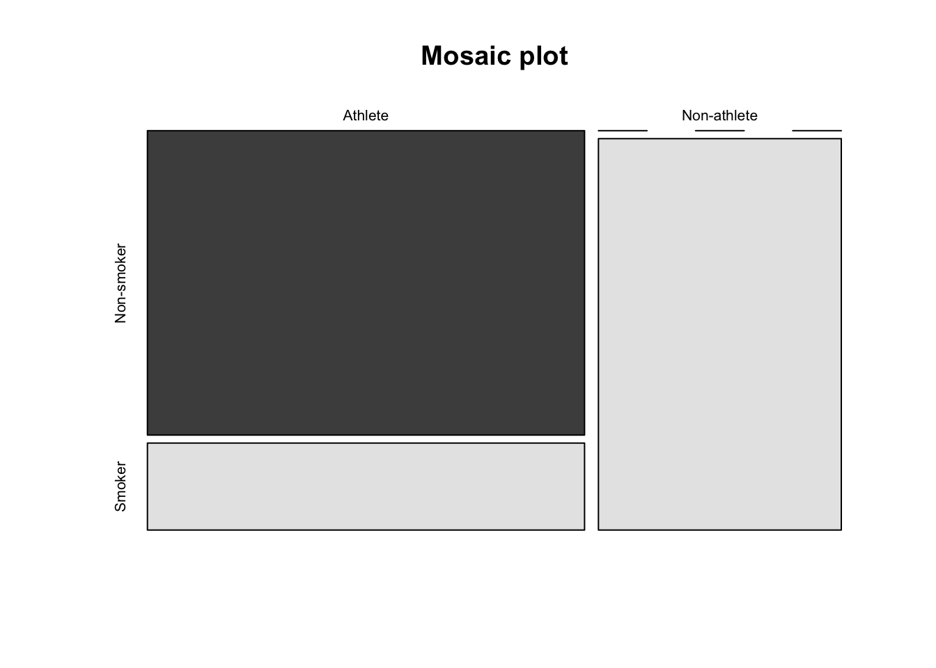
We can already see from the plot that the proportion of smokers in the sample is higher among non-athletes than athlete. The plot is however not sufficient to conclude that there is such a significant association in the population.
Like many statistical tests, this can be done via a hypothesis test. But before seeing how to do it in R, let’s see the concept of expected frequencies.
Expected frequencies
Remember that the Fisher’s exact test is used when there is at least one cell in the contingency table of the expected frequencies below 5. To retrieve the expected frequencies, use the chisq.test() function together with $expected:
chisq.test(dat)$expected## Warning in chisq.test(dat): Chi-squared approximation may be incorrect## Non-smoker Smoker
## Athlete 4.5 4.5
## Non-athlete 2.5 2.5The contingency table above confirms that we should use the Fisher’s exact test instead of the Chi-square test because there is at least one cell below 5.
Tip: although it is a good practice to check the expected frequencies before deciding between the Chi-square and the Fisher test, it is not a big issue if you forget. As you can see above, when doing the Chi-square test in R (with chisq.test()), a warning such as “Chi-squared approximation may be incorrect” will appear. This warning means that the smallest expected frequencies is lower than 5. Therefore, do not worry if you forgot to check the expected frequencies before applying the appropriate test to your data, R will warn you that you should use the Fisher’s exact test instead of the Chi-square test if that is the case.
(Remember that, as for the Chi-square test of independence, the observations must be independent in order for the Fisher’s exact test to be valid. See more details about the independence assumption in this section.)
Fisher’s exact test in R
To perform the Fisher’s exact test in R, use the fisher.test() function as you would do for the Chi-square test:
test <- fisher.test(dat)
test
##
## Fisher's Exact Test for Count Data
##
## data: dat
## p-value = 0.02098
## alternative hypothesis: true odds ratio is not equal to 1
## 95 percent confidence interval:
## 1.449481 Inf
## sample estimates:
## odds ratio
## InfThe most important in the output is the \(p\)-value. You can also retrieve the \(p\)-value with:
test$p.value## [1] 0.02097902Note that if your data is not already presented as a contingency table, you can simply use the following code:
fisher.test(table(dat$variable1, dat$variable2))where dat is the name of your dataset, variable1 and variable2 correspond to the names of the two variables of interest.
Conclusion and interpretation
From the output and from test$p.value we see that the \(p\)-value is less than the significance level of 5%. Like any other statistical test, if the \(p\)-value is less than the significance level, we can reject the null hypothesis. If you are not familiar with \(p\)-values, I invite you to read this section.
\(\Rightarrow\) In our context, rejecting the null hypothesis for the Fisher’s exact test of independence means that there is a significant relationship between the two categorical variables (smoking habits and being an athlete or not). Therefore, knowing the value of one variable helps to predict the value of the other variable.
Combination of plot and statistical test
It is possible print the results of the Fisher’s exact test directly on a barplot thanks to the ggbarstats() function from the {ggstatsplot} package (the function has been slightly edited to match our needs).
It is easier to work with the package when our data is not already in the form of a contingency table so we transform it to a data frame before plotting the results:
# create dataframe from contingency table
x <- c()
for (row in rownames(dat)) {
  for (col in colnames(dat)) {
    x <- rbind(x, matrix(rep(c(row, col), dat[row, col]), ncol = 2, byrow = TRUE))
  }
}
df <- as.data.frame(x)
colnames(df) <- c("Sport_habits", "Smoking_habits")
df
## Sport_habits Smoking_habits
## 1 Athlete Non-smoker
## 2 Athlete Non-smoker
## 3 Athlete Non-smoker
## 4 Athlete Non-smoker
## 5 Athlete Non-smoker
## 6 Athlete Non-smoker
## 7 Athlete Non-smoker
## 8 Athlete Smoker
## 9 Athlete Smoker
## 10 Non-athlete Smoker
## 11 Non-athlete Smoker
## 12 Non-athlete Smoker
## 13 Non-athlete Smoker
## 14 Non-athlete Smoker# Fisher's exact test with raw data
test <- fisher.test(table(df))
# combine plot and statistical test with ggbarstats
library(ggstatsplot)
ggbarstats(
df, Smoking_habits, Sport_habits,
results.subtitle = FALSE,
subtitle = paste0(
"Fisher's exact test", ", p-value = ",
ifelse(test$p.value < 0.001, "< 0.001", round(test$p.value, 3))
)
)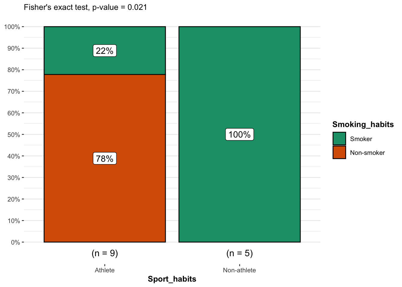
From the plot, it is clear that the proportion of smokers among non-athletes is higher than among athletes, suggesting that there is a relationship between the two variables.
This is confirmed thanks to the \(p\)-value displayed in the subtitle of the plot. As previously, we reject the null hypothesis and we conclude that the variables smoking habits and being an athlete or not are dependent (\(p\)-value = 0.021).
Conclusion
Thanks for reading.
I hope the article helped you to perform the Fisher’s exact test of independence in R and interpret its results. Learn more about the Chi-square test of independence by hand or in R.
As always, if you have a question or a suggestion related to the topic covered in this article, please add it as a comment so other readers can benefit from the discussion.
References
The data are the same than for the article covering the Chi-square test by hand, except that some observations have been removed to decrease the sample size.↩︎
Liked this post?
- Get updates every time a new article is published (no spam and unsubscribe anytime)
- Support the blog
- Share on:


