
Wilcoxon test in R: how to compare 2 groups under the non-normality assumption?

Introduction
In a previous article, we showed how to compare two groups under different scenarios using the Student’s t-test. The Student’s t-test requires that the distributions follow a normal distribution when in presence of small samples.1
In this article, we show how to compare two groups when the normality assumption is violated, using the Wilcoxon test.
The Wilcoxon test is a non-parametric test, meaning that it does not rely on data belonging to any particular parametric family of probability distributions. Non-parametric tests have the same objective as their parametric counterparts. However, they have two advantages over parametric tests: they do not require the assumption of normality of distributions and they can deal with outliers.
A Student’s t-test for instance is only applicable if the data are Gaussian or if the sample size is large enough (usually \(n \ge 30\), thanks to the central limit theorem). A non-parametric test should be used in other cases.
One may wonder why we would not always use a non-parametric test so we do not have to bother about testing for normality. The reason is that non-parametric tests are usually less powerful than corresponding parametric tests when the normality assumption holds.
Therefore, all else being equal, with a non-parametric test you are less likely to reject the null hypothesis when it is false if the data follows a normal distribution. It is thus preferred to use the parametric version of a statistical test when the assumptions are met.
In the remaining of the article, we present the two scenarios of the Wilcoxon test and how to perform them in R through two examples.
Two different scenarios
As for the Student’s t-test, the Wilcoxon test is used to compare two groups and see whether they are significantly different from each other in terms of the variable of interest.
The two groups to be compared are either:
- independent, or
- paired (i.e., dependent)
There are actually two versions of the Wilcoxon test:
- The Mann-Whitney-Wilcoxon test (also referred as Wilcoxon rank sum test or Mann-Whitney U test) is performed when the samples are independent (so this test is the non-parametric equivalent to the Student’s t-test for independent samples).
- The Wilcoxon signed-rank test (also sometimes referred as Wilcoxon test for paired samples) is performed when the samples are paired/dependent (so this test is the non-parametric equivalent to the Student’s t-test for paired samples).
Luckily, those two tests can be done in R with the same function: wilcox.test(). They are presented in the following sections.
Independent samples
For the Wilcoxon test with independent samples, suppose that we want to test whether grades at the statistics exam differ between female and male students.
We have collected grades for 24 students (12 girls and 12 boys):
dat <- data.frame(
  Sex = as.factor(c(rep("Girl", 12), rep("Boy", 12))),
  Grade = c(
    19, 18, 9, 17, 8, 7, 16, 19, 20, 9, 11, 18,
    16, 5, 15, 2, 14, 15, 4, 7, 15, 6, 7, 14
  )
)

dat
## Sex Grade
## 1 Girl 19
## 2 Girl 18
## 3 Girl 9
## 4 Girl 17
## 5 Girl 8
## 6 Girl 7
## 7 Girl 16
## 8 Girl 19
## 9 Girl 20
## 10 Girl 9
## 11 Girl 11
## 12 Girl 18
## 13 Boy 16
## 14 Boy 5
## 15 Boy 15
## 16 Boy 2
## 17 Boy 14
## 18 Boy 15
## 19 Boy 4
## 20 Boy 7
## 21 Boy 15
## 22 Boy 6
## 23 Boy 7
## 24 Boy 14Here are the distributions of the grades by sex (using {ggplot2}):
library(ggplot2)

ggplot(dat) +
  aes(x = Sex, y = Grade) +
  geom_boxplot(fill = "#0c4c8a") +
  theme_minimal()
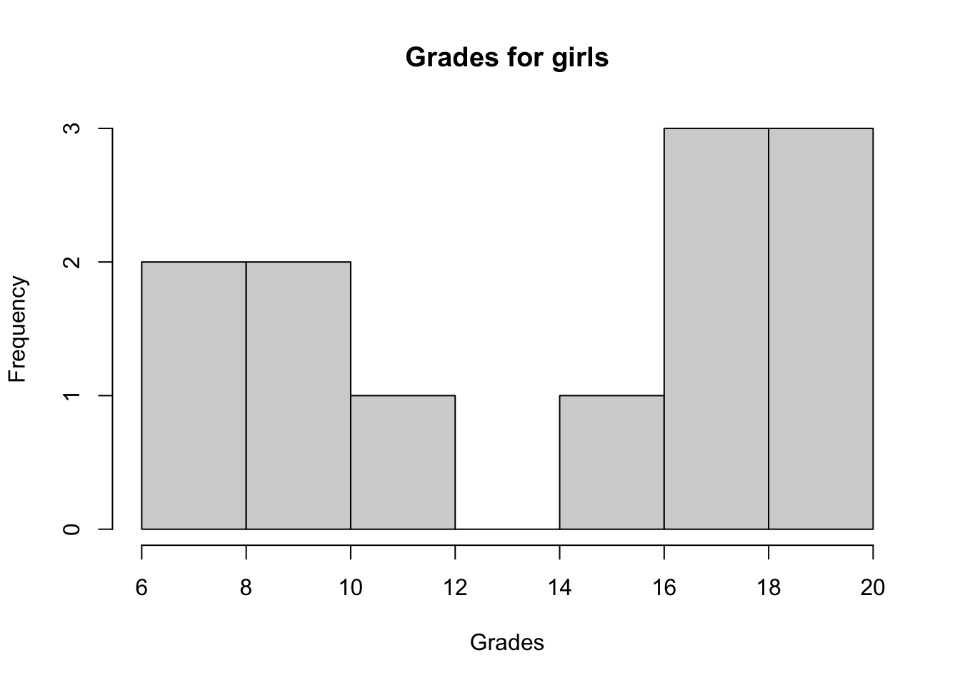
We first check whether the 2 samples follow a normal distribution via a histogram and the Shapiro-Wilk test:
hist(subset(dat, Sex == "Girl")$Grade,
  main = "Grades for girls",
  xlab = "Grades"
)
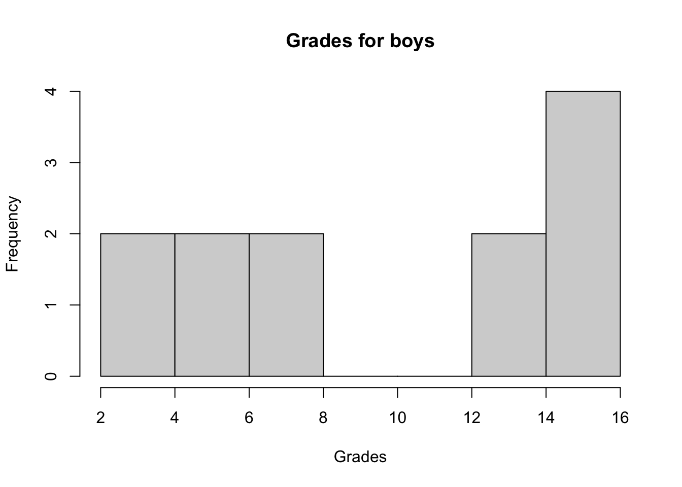
hist(subset(dat, Sex == "Boy")$Grade,
  main = "Grades for boys",
  xlab = "Grades"
)
shapiro.test(subset(dat, Sex == "Girl")$Grade)##
## Shapiro-Wilk normality test
##
## data: subset(dat, Sex == "Girl")$Grade
## W = 0.84548, p-value = 0.0323shapiro.test(subset(dat, Sex == "Boy")$Grade)##
## Shapiro-Wilk normality test
##
## data: subset(dat, Sex == "Boy")$Grade
## W = 0.84313, p-value = 0.03023The histograms show that both distributions do not seem to follow a normal distribution and the p-values of the Shapiro-Wilk tests confirm it (since we reject the null hypothesis of normality for both distributions at the 5% significance level).
We just showed that normality assumption is violated for both groups so it is now time to see how to perform the Wilcoxon test in R.
Note that in order to use the Student’s t-test (the parametric version of the Wilcoxon test), it is required that both samples follow a normal distribution if samples are small.2 Therefore, even if one sample follows a normal distribution (and the other does not follow a normal distribution), it is recommended to use the non-parametric test.
Remember that the null and alternative hypothesis of the Wilcoxon test are as follows:
- \(H_0\): the 2 groups are equal in terms of the variable of interest
- \(H_1\): the 2 groups are different in terms of the variable of interest
Applied to our research question, we have:
- \(H_0\): grades of girls and boys are equal
- \(H_1\): grades of girls and boys are different
test <- wilcox.test(dat$Grade ~ dat$Sex)
test
##
## Wilcoxon rank sum test with continuity correction
##
## data: dat$Grade by dat$Sex
## W = 31.5, p-value = 0.02056
## alternative hypothesis: true location shift is not equal to 0We obtain the test statistic, the p-value and a reminder of the hypothesis tested.3
The p-value is 0.021. Therefore, at the 5% significance level, we reject the null hypothesis and we conclude that grades are significantly different between girls and boys.
Given the boxplot presented above showing the grades by sex, one may see that girls seem to perform better than boys. This can be tested formally by adding the alternative = "less" argument to the wilcox.test() function:4
test <- wilcox.test(dat$Grade ~ dat$Sex,
  alternative = "less"
)
test
##
## Wilcoxon rank sum test with continuity correction
##
## data: dat$Grade by dat$Sex
## W = 31.5, p-value = 0.01028
## alternative hypothesis: true location shift is less than 0The p-value is 0.01. Therefore, at the 5% significance level, we reject the null hypothesis and we conclude that boys performed significantly worse than girls (which is equivalent than concluding that girls performed significantly better than boys).
Paired samples
For this second scenario, consider that we administered a math test in a class of 12 students at the beginning of a semester, and that we administered a similar test at the end of the semester to the exact same students. We have the following data:
dat2 <- data.frame(
  Beginning = c(16, 5, 15, 2, 14, 15, 4, 7, 15, 6, 7, 14),
  End = c(19, 18, 9, 17, 8, 7, 16, 19, 20, 9, 11, 18)
)

dat2
## Beginning End
## 1 16 19
## 2 5 18
## 3 15 9
## 4 2 17
## 5 14 8
## 6 15 7
## 7 4 16
## 8 7 19
## 9 15 20
## 10 6 9
## 11 7 11
## 12 14 18We transform the dataset to have it in a tidy format:
dat2 <- data.frame(
  Time = c(rep("Before", 12), rep("After", 12)),
  Grade = c(dat2$Beginning, dat2$End)
)
dat2
## Time Grade
## 1 Before 16
## 2 Before 5
## 3 Before 15
## 4 Before 2
## 5 Before 14
## 6 Before 15
## 7 Before 4
## 8 Before 7
## 9 Before 15
## 10 Before 6
## 11 Before 7
## 12 Before 14
## 13 After 19
## 14 After 18
## 15 After 9
## 16 After 17
## 17 After 8
## 18 After 7
## 19 After 16
## 20 After 19
## 21 After 20
## 22 After 9
## 23 After 11
## 24 After 18The distribution of the grades at the beginning and after the semester:
# Reordering dat2$Time
dat2$Time <- factor(dat2$Time,
  levels = c("Before", "After")
)

ggplot(dat2) +
  aes(x = Time, y = Grade) +
  geom_boxplot(fill = "#0c4c8a") +
  theme_minimal()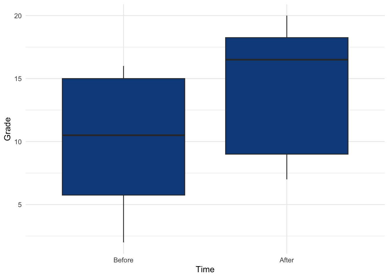
(See the {esquisse} and {questionr} addins to help you reorder levels of a factor variable and to easily draw plots with the {ggplot2} package.)
In this example, it is clear that the two samples are not independent since the same 12 students took the exam before and after the semester. Supposing also that the normality assumption is violated (and given the small sample size), we thus use the Wilcoxon test for paired samples, with the following hypotheses:5
- \(H_0\): grades before and after the semester are equal
- \(H_1\): grades before and after the semester are different
We add the paired = TRUE argument to the wilcox.test() function to take into consideration the dependency between the 2 samples:
before <- dat2$Grade[dat2$Time == "Before"]
after <- dat2$Grade[dat2$Time == "After"]
test <- wilcox.test(before, after, paired = TRUE)

test
##
## Wilcoxon signed rank test with continuity correction
##
## data: before and after
## V = 21, p-value = 0.1692
## alternative hypothesis: true location shift is not equal to 0We obtain the test statistic, the p-value and a reminder of the hypothesis tested.
The p-value is 0.169. Therefore, at the 5% significance level, we do not reject the null hypothesis that the grades are similar before and after the semester.
Combination of plot and statistical test
After having written this article, I discovered the {ggstatsplot} package which I believe is worth mentioning here, in particular the ggbetweenstats() and ggwithinstats() functions for independent and paired samples, respectively.
These two functions combine a boxplot—representing the distribution for each group—and the results of the statistical test displayed in the subtitle of the plot.
See examples below for independent and paired samples, using the same data than previously.
Independent samples
For independent samples, it is the ggbetweenstats() function which is used:
# load package
library(ggstatsplot)

# plot with statistical results
ggbetweenstats( # independent samples
  data = dat,
  x = Sex,
  y = Grade,
  plot.type = "box", # for boxplot
  type = "nonparametric", # for wilcoxon
  centrality.plotting = FALSE # remove median
)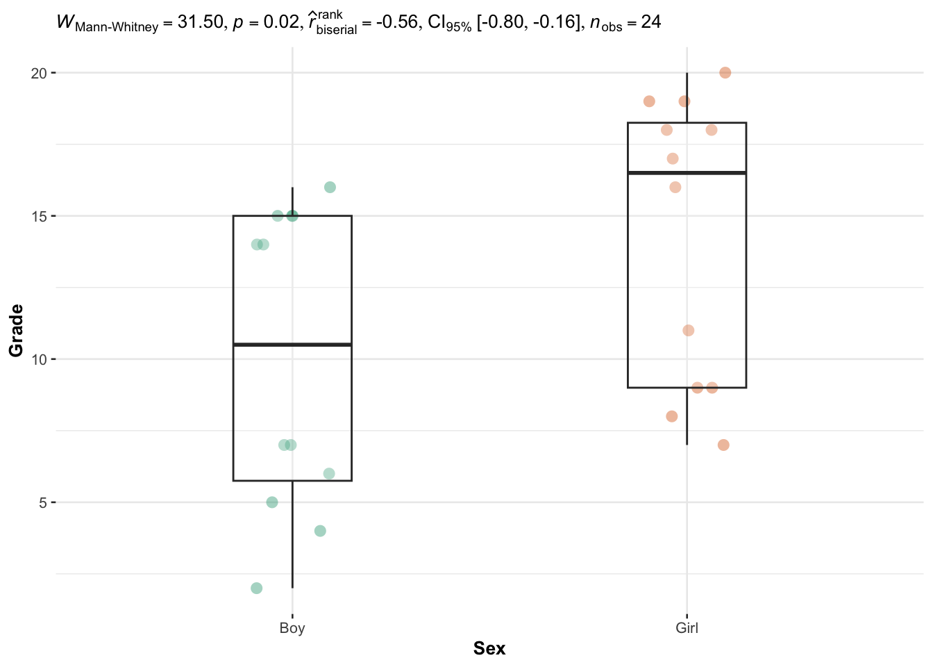
The p-value (displayed after p = in the subtitle of the plot) indicates that we reject the null hypothesis, and we conclude that grades are significantly different between girls and boys (p-value = 0.02).
Paired samples
For paired samples, it is the ggwithinstats() function which is used:
# load package
library(ggstatsplot)

# plot with statistical results
ggwithinstats( # paired samples
  data = dat2,
  x = Time,
  y = Grade,
  type = "nonparametric", # for wilcoxon
  centrality.plotting = FALSE # remove median
)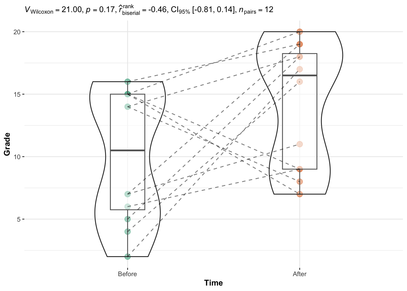
The p-value (displayed after p = in the subtitle of the plot) indicates that we do not reject the null hypothesis, so we do not reject the hypothesis that grades are equal before and after the semester (p-value = 0.17).
The point of this section was to illustrate how to easily draw plots together with statistical results, which is exactly the aim of the {ggstatsplot} package. See more details and examples in this article.
Assumption of equal variances
As written at the beginning of the article, the Wilcoxon test does not require the assumption of normality in case of small samples.
Regarding the assumption of equal variances, this assumption may or may not be needed depending on your goal. If you only want to compare the two groups, you do not have to test the equality of variances because the two distributions do not have to have the same shape. However, if your goal is to compare medians of the two groups, then you will need to make sure that the two distributions have the same shape (and thus, the same variance).6
So results of your test of equality of variances will change your interpretation: differences in the “distributions” of two groups or differences in the “medians” of two groups.
In this article I do not wish to compare medians, I only want compare the groups by determining whether there are differences in the distributions of the two groups. This is the reason I do not test for equality of variances.
Note that this is equivalent when performing the Kruskal-Wallis test to compare three groups or more (i.e., the non-parametric version of the ANOVA): if you only want to test whether there are differences in the groups you do not need homoscedasticity, whereas if you want to compare the medians this assumption must be met.
Conclusion
Thanks for reading.
I hope this article helped you to compare two groups that do not follow a normal distribution in R using the Wilcoxon test. See also:
- the one-sample Wilcoxon test if you have only one group and want to compare it to a default given value,
- the Student’s t-test if you need to perform the parametric version of the two-sample Wilcoxon test,
- and the ANOVA if you need to compare 3 groups or more.
As always, if you have a question or a suggestion related to the topic covered in this article, please add it as a comment so other readers can benefit from the discussion.
References
Remember that the normality assumption can be tested via 3 complementary methods: (i) histogram, (ii) QQ-plot and (iii) normality tests (with the most common being the Shapiro-Wilk test). See how to determine if a distribution follows a normal distribution if you need a refresh.↩︎
In case of large samples, normality is not required (this is a common misconception!). By the central limit theorem, sample means of large samples are often well-approximated by a normal distribution even if the data are not normally distributed (Stevens 2013).↩︎
Note that the presence of equal elements (ties) prevents an exact p-value calculation. This can be tackled by computing the exact or asymptotic Wilcoxon-Mann-Whitney test with adjustment for ties, using the
wilcox_test()function from the{coin}package:wilcox_test(dat$Grade ~ dat$Sex, distribution = exact())orwilcox_test(dat$Grade ~ dat$Sex). In our case, conclusions remain unchanged.↩︎We add
alternative = "less"(and notalternative = "greater") because we want to test that grades for boys are less than grade for girls. Using"less"or"greater"can be deducted from the reference level in the dataset.↩︎Note that for paired samples (when in presence of a small sample), normality must be checked on the differences between the two paired samples, and not individually on the two samples like it is done for independent samples.↩︎
See these three articles for a more detailed discussion on the assumption of equal variances in Wilcoxon test: 1, 2 & 3.↩︎
Liked this post?
- Get updates every time a new article is published (no spam and unsubscribe anytime)
- Support the blog
- Share on:


