
Kruskal-Wallis test, or the nonparametric version of the ANOVA

Introduction
In a previous article, we showed how to do an ANOVA in R to compare three or more groups.
Remember that, as for many statistical tests, the one-way ANOVA requires that some assumptions are satisfied in order to be able to use and interpret the results. In particular, the ANOVA requires that residuals follow approximately a normal distribution.1
Luckily, if the normality assumption is not satisfied, there is the nonparametric version of the ANOVA: the Kruskal-Wallis test.
In the rest of the article, we show how to perform the Kruskal-Wallis test in R and how to interpret its results. We will also briefly show how to do post-hoc tests and how to present all necessary statistical results directly on a plot.
Data
Data for the present article is based on the penguins dataset (an alternative to the well-known iris dataset), accessible via the {palmerpenguins} package:
# install.packages("palmerpenguins")
library(palmerpenguins)
The original dataset contains data for 344 penguins of 3 different species (Adelie, Chinstrap and Gentoo).
It contains 8 variables, but we focus only on the flipper length and the species for this article, so we keep only those 2 variables:
library(tidyverse)

dat <- penguins %>%
  select(species, flipper_length_mm)
(If you are unfamiliar with the pipe operator (%>%), you can also select variables with penguins[, c("species", "flipper_length_mm")]. Learn more ways to select variables in the article about data manipulation.)
It is always a good practice to do some descriptive statistics for the entire sample and by group before doing the test, so we have a broad overview of the data at hand.
# entire sample
summary(dat)
## species flipper_length_mm
## Adelie :152 Min. :172.0
## Chinstrap: 68 1st Qu.:190.0
## Gentoo :124 Median :197.0
## Mean :200.9
## 3rd Qu.:213.0
## Max. :231.0
## NA's :2# by group
library(doBy)
summaryBy(flipper_length_mm ~ species,
data = dat,
FUN = median,
na.rm = TRUE
)## # A tibble: 3 × 2
## species flipper_length_mm.median
## <fct> <dbl>
## 1 Adelie 190
## 2 Chinstrap 196
## 3 Gentoo 216# boxplot by species
ggplot(dat) +
aes(x = species, y = flipper_length_mm, fill = species) +
geom_boxplot() +
theme(legend.position = "none")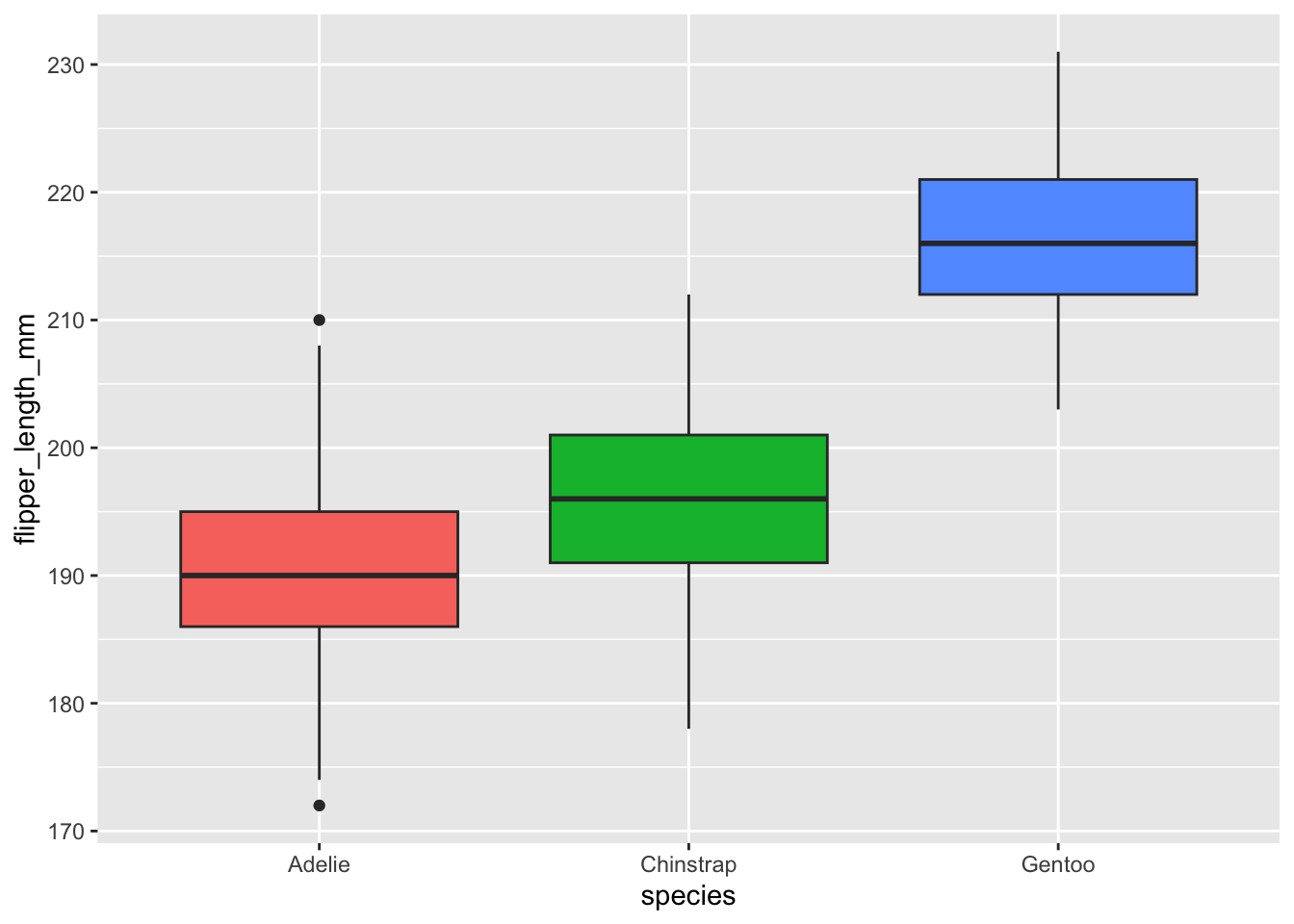
Based on the boxplots and the summary statistics, we already see that, in our sample, penguins from the Adelie species seem to have the smallest flippers, while those from the Gentoo species seem to have the biggest flippers. However, only a sound statistical test will tell us whether we can infer this conclusion to our population.
Kruskal-Wallis test
Aim and hypotheses
As mentioned earlier, the Kruskal-Wallis test allows to compare three or more groups. More precisely, it is used to compare three or more groups in terms of a quantitative variable.
It can be seen as the extension to the Mann-Whitney test which allows to compare 2 groups under the non-normality assumption.
In the context of our example, we are going to use the Kruskal-Wallis test to help us answer the following question: “Is the length of the flippers different between the 3 species of penguins?”.
The null and alternative hypotheses of the Kruskal-Wallis test are:
- \(H_0\): The 3 species are equal in terms of flipper length
- \(H_1\): At least one species is different from the other 2 species in terms of flipper length
Be careful that, as for the ANOVA, the alternative hypothesis is not that all species are different in terms of flipper length. The opposite of all species being equal (\(H_0\)) is that at least one species is different from the others (\(H_1\)).
In this sense, if the null hypothesis is rejected, it means that at least one species is different from the other 2, but not necessarily that all 3 species are different from each other. It could be that flipper length for the species Gentoo is different than for the species Chinstrap and Adelie, but flipper length is similar between Chinstrap and Adelie. Other types of test (known as post-hoc tests and covered later) must be performed to test whether all 3 species differ.
Assumptions
First, the Kruskal-Wallis test compares several groups in terms of a quantitative variable. So there must be one quantitative dependent variable (which corresponds to the measurements to which the question relates) and one qualitative independent variable (with at least 2 levels which will determine the groups to compare).2
Second, remember that the Kruskal-Wallis test is a nonparametric test, so the normality assumption is not required. However, the independence assumption still holds.
This means that the data, collected from a representative and randomly selected portion of the total population, should be independent between groups and within each group. The assumption of independence is most often verified based on the design of the experiment and on the good control of experimental conditions rather than via a formal test. If you are still unsure about independence based on the experiment design, ask yourself if one observation is related to another (if one observation has an impact on another) within each group or between the groups themselves. If not, it is most likely that you have independent samples. If observations between samples (forming the different groups to be compared) are dependent (for example, if three measurements have been collected on the same individuals as it is often the case in medical studies when measuring a metric (i) before, (ii) during and (iii) after a treatment), the Friedman test should be preferred in order to take into account the dependency between the samples.
Regarding the homoscedasticity (i.e., equality of the variances): As long as you use the Kruskal-Wallis test to, in fine, compare groups, homoscedasticity is not required. If you wish to compare medians, the Kruskal-Wallis test requires homoscedasticity.3
In our example, independence is assumed and we do not need to compare medians (we are only interested in comparing groups), so we can proceed to how to do the test in R. Note that the normality assumption may or may not hold, but for this article we assume it is not satisfied.
In R
The Kruskal-Wallis test in R can be done with the kruskal.test() function:
kruskal.test(flipper_length_mm ~ species,
  data = dat
)
##
## Kruskal-Wallis rank sum test
##
## data: flipper_length_mm by species
## Kruskal-Wallis chi-squared = 244.89, df = 2, p-value < 2.2e-16The most important result in this output is the p-value. We show how to interpret it in the next section.
Interpretations
Based on the Kruskal-Wallis test, we reject the null hypothesis and we conclude that at least one species is different in terms of flippers length (p-value < 0.001).
(For the sake of illustration, if the p-value was larger than the significance level \(\alpha = 0.05\): we cannot reject the null hypothesis so we cannot reject the hypothesis that the 3 considered species of penguins are equal in terms of flippers length.)
Post-hoc tests
We have just showed that at least one species is different from the others in terms of flippers length. Nonetheless, here comes the limitations of the Kruskal-Wallis test: it does not say which group(s) is(are) different from the others.
To know this, we need to use other types of test, referred as post-hoc tests (in Latin, “after this”, so after obtaining statistically significant Kruskal-Wallis results) or multiple pairwise-comparison tests. For the interested reader, a more detailed explanation of post-hoc tests can be found here.
The most common post-hoc tests after a significant Kruskal-Wallis test are:
- Dunn test
- Conover test
- Nemenyi test
- Pairwise Wilcoxon test
The Dunn test being the most common one, here is how to do it in R.4
Dunn test
library(FSA)

dunnTest(flipper_length_mm ~ species,
  data = dat,
  method = "holm"
)
## Comparison Z P.unadj P.adj
## 1 Adelie - Chinstrap -3.629336 2.841509e-04 2.841509e-04
## 2 Adelie - Gentoo -15.476612 4.990733e-54 1.497220e-53
## 3 Chinstrap - Gentoo -8.931938 4.186100e-19 8.372200e-19It is the last column (the adjusted p-values, adjusted for multiple comparisons) that is of interest. These p-values should be compared to your desired significance level (usually 5%).
Based on the output, we conclude that:
- Adelie and Chinstrap differ significantly (p < 0.001)
- Adelie and Gentoo differ significantly (p < 0.001)
- Chinstrap and Gentoo differ significantly (p < 0.001)
Therefore, based on the Dunn test, we can now conclude that all 3 species differ in terms of flipper length.
Combination of statistical results and plot
A very good alternative for performing a Kruskal-Wallis and the post-hoc tests in R is with the ggbetweenstats() function from the {ggstatsplot} package:
library(ggstatsplot)

ggbetweenstats(
  data = dat,
  x = species,
  y = flipper_length_mm,
  type = "nonparametric", # ANOVA or Kruskal-Wallis
  plot.type = "box",
  pairwise.comparisons = TRUE,
  pairwise.display = "significant",
  centrality.plotting = FALSE,
  bf.message = FALSE
)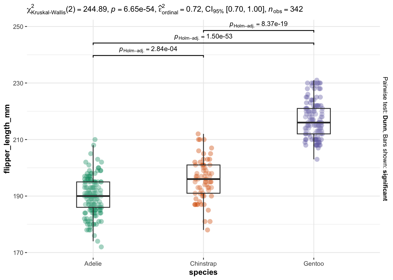
This method has the advantage that all necessary statistical results are displayed directly on the plot.
The results of the Kruskal-Wallis test are shown in the subtitle above the plot (the p-value is after p =). Moreover, the results of the post-hoc test are displayed between each group via accolades, and the boxplots allow to visualize the distribution for each species.
Summary
In this post, we reviewed the aim and hypotheses of the Kruskal-Wallis test and its underlying assumptions. We then showed how to do the test in R and how to interpret the results.
We also showed the most common post-hoc test after a significant Kruskal-Wallis test—the Dunn test.
Last but not least, we presented a concise way to present both the data by group and all the statistical results on the same plot.
Thanks for reading.
As always, if you have a question or a suggestion related to the topic covered in this article, please add it as a comment so other readers can benefit from the discussion.
References
This is the case for small sample sizes. For large sample sizes, normality is not required (this is a common misconception!). By the central limit theorem, sample means of large samples are often well-approximated by a normal distribution even if the data are not normally distributed (Stevens 2013). See more details in this note.↩︎
Note that in theory, Kruskal-Wallis test can also be used for only two groups. However, in practice we use the Mann-Whitney test for two groups and Kruskal-Wallis for three or more groups.↩︎
See more information about the difference in this article.↩︎
Note that there are other p-value adjustment methods. See
?dunnTestfor more options.↩︎
Liked this post?
- Get updates every time a new article is published (no spam and unsubscribe anytime)
- Support the blog
- Share on:


