
Descriptive statistics by hand

Introduction
This article explains how to compute the main descriptive statistics by hand and how to interpret them. To learn how to compute these measures in R, read the article “Descriptive statistics in R”.
Descriptive statistics (in the broad sense of the term) is a branch of statistics aiming at summarizing, describing and presenting a series of values or a dataset. Long series of values without any preparation or without any summary measures are often not informative due to the difficulty of recognizing any pattern in the data. Below an example with the height (in cm) of a population of 100 adults:
188.7, 169.4, 178.6, 181.3, 179, 173.9, 190.1, 174.1, 195.2, 174.4, 188, 197.9, 161.1, 172.2, 173.7, 181.4, 172.2, 148.4, 150.6, 188.2, 171.9, 157.2, 173.3, 187.1, 194, 170.7, 172.4, 157.4, 179.6, 168.6, 179.6, 182, 185.4, 168.9, 180, 157.8, 167.2, 166.5, 150.9, 175.4, 177.1, 171.4, 182.6, 167.7, 161.3, 179.3, 166.9, 189.4, 170.7, 181.6, 178.2, 167.2, 190.8, 181.4, 175.9, 177.8, 181.8, 175.9, 145.1, 177.8, 171.3, 176.9, 180.8, 189, 167.7, 188, 178.4, 185.4, 184.2, 182.2, 164.6, 174.1, 181.2, 165.5, 169.6, 180.8, 182.7, 179.6, 166.1, 164, 190.1, 177.6, 175.9, 173.8, 163.1, 181.1, 172.8, 173.2, 184.3, 183.2, 188.9, 170.2, 181.5, 188.9, 163.9, 166.4, 163.7, 160.4, 175.8 and 181.5
Facing this series, it is hard (not to say impossible) for anyone to understand the data and have a clear view of the size of these adults in a reasonable amount of time. Descriptive statistics allow to summarize, and thus have a better overview of the data. Of course, by summarizing data through one or several measures, some information will inevitably be lost. However, in many cases it is generally better to lose some information but in return gain an overview.
Descriptive statistics is often the first step and an important part in any statistical analysis. It allows to check the quality of the data by detecting potential outliers (i.e., data points that appear to be separated from the rest of the data), collection or encoding errors. It also helps to “understand” the data and if well presented, descriptive statistics is already a good starting point for further analyses.
Location versus dispersion measures
Several different measures (called statistics if we are analyzing a sample) are used to summarize the data. Some of them give an understanding about the location of the data, others give and understanding about the dispersion of the data. In practice, both types of measures are often used together in order to summarize the data in the most concise but complete way.
We illustrate this point with the graph below, representing the height (in cm) of 100 persons divided into two groups (50 persons in each group):
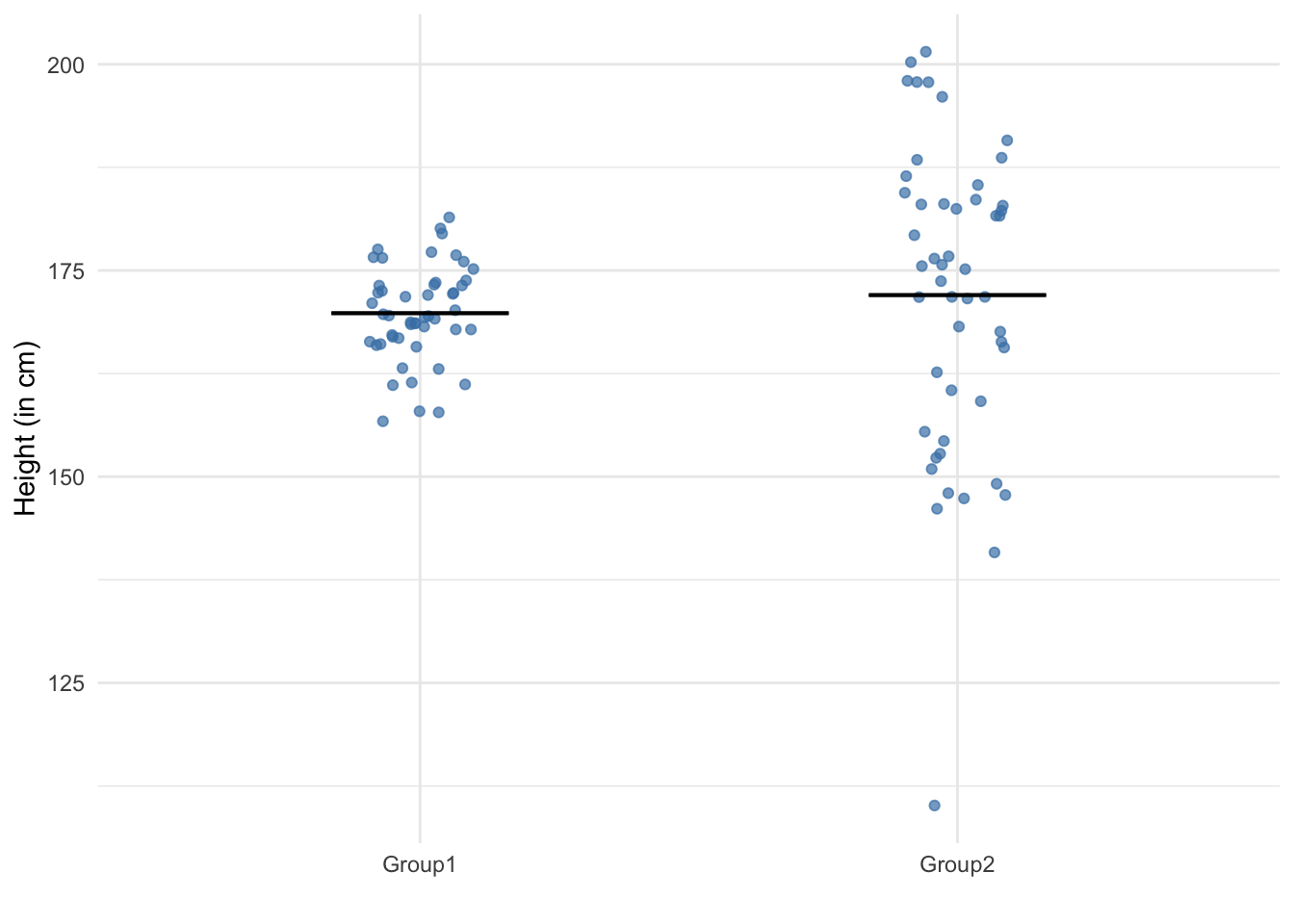
The black line corresponds to the mean. The mean height (in cm) is similar in both groups. However, it is clear that the dispersion of heights are very different in the two groups. For this reason, location or dispersion measures are often not enough if presented individually and it is a good practice to present several statistics from both types of measures.
In the following sections, we detail the most common location and dispersion measures and illustrate them with examples. Note that for the sake of simplicity, we consider only series of values (i.e., univariate data) and not bivariate or multivariate data, and we do not consider the case of series grouped in classes.
Location
Location measures allow to see “where” the data are located, around which values. In other words, location measures give an understanding on what is the central tendency, the “position” of the data as a whole. It includes the following statistics (others exist but we focus on the most common ones):
- minimum
- maximum
- mean
- median
- first quartile
- third quartile
- mode
We detail and compute by hand each of them in the following sections.
Minimum and maximum
Minimum (\(min\)) and maximum (\(max\)) are simply the lowest and largest values, respectively. Given the height (in cm) of a sample of 6 adults:
188.7, 169.4, 178.6, 181.3, 179 and 173.9
The minimum is 169.4 cm and the maximum is 188.7 cm. These two basic statistics give a clear idea about the size of the smallest and tallest of these 6 adults.
Mean
The mean, also known as average, is probably the most common statistics. It gives an idea on what is the average value, that is, the central value of the data or in other words the center of gravity:1
The mean is found by summing all values and dividing the total by the number of observations (denoted \(n\)):
\[mean = \bar{x} = \frac{\text{sum of all values}}{\text{number of values}} = \frac{1}{n}\sum^{n}_{i = 1} x_i\]
Given our sample of 6 adults presented above, the mean is:
\[\bar{x} = \frac{188.7 + 169.4 + 178.6}{6}\] \[\frac{+ 181.3 + 179 + 173.9}{6}\\ = 178.4833\]
In conclusion, the mean size, that is, the average size of our sample of 6 adults is 178.48 cm (rounded to 2 decimals).
Median
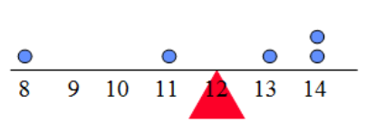
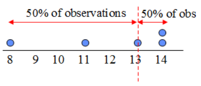
The median is another measure of location so it also gives an idea about the central tendency of the data. The interpretation of the median is that there are as many observations below as above the median. In other words, 50% of the observations lie below the median, and 50% of the observations lie above the median. Below a visual representation of the median:
The easiest way to compute the median is by first sorting the data from lowest to highest (i.e., in ascending order) then take the middle point as the median. From the sorted values, for an odd number of observations, the middle point is easy to find: it is the value with as many observations below as above. Still from the sorted values, for an even number of observations, the middle point is exactly between the two middle values. Formally, after sorting, the median is:
- if \(n\) (number of observations) is odd: \[med(x) = x_{\frac{n+1}{2}}\]
- if \(n\) is even: \[med(x) = \frac{1}{2}\big(x_{\frac{n}{2}} + x_{\frac{n}{2} + 1}\big)\]
where the subscript of \(x\) denotes the numbering of the sorted data. The formulas look harder than they really are, so let’s see with two concrete examples.
Odd number of observations
Given the height of a sample of 7 adults taken from the 100 adults presented in the introduction:
188.9, 163.9, 166.4, 163.7, 160.4, 175.8 and 181.5
We first sort the order from lowest to highest:
160.4, 163.7, 163.9, 166.4, 175.8, 181.5 and 188.9
Given that the number of observations \(n\) is odd (since \(n = 7\)), the median is
\[med(x) = x_\frac{7 + 1}{2} = x_4\]
So we take the fourth value from the sorted values, which corresponds to 166.4. In conclusion, the median size of these 7 adults is 166.4 cm. As you can see, there are 3 observations below 166.4 and 3 observations above 166.4 cm.
Even number of observations
Now let’s see when the number of observations is even, which is slightly more complicated than when the number of observations is odd. Given the height of a sample of 6 adults:
188.7, 169.4, 178.6, 181.3, 179 and 173.9
We sort the values in ascending order:
169.4, 173.9, 178.6, 179, 181.3 and 188.7
Given that the number of observations \(n\) is even (since \(n = 6\)), the median is
\[med(x) = \frac{1}{2}\big(x_{\frac{6}{2}} + x_{\frac{6}{2} + 1}\big) = \frac{1}{2}\big(x_{3} + x_{4}\big)\]
So we sum the third and fourth values from the sorted values and divide the total by 2 (which is equivalent than taking the mean of these two middle values):
\[\frac{1}{2}(178.6 + 179) = 178.8\]
In conclusion, the median size of these 6 adults is 178.8 cm. Again, remark that there are as many observations below as above 178.8 cm.
Mean vs. median
Although the mean and median are often relatively close to each other (in particular when the distribution is symmetric) they should not be confused since they both have advantages and disadvantages in different contexts. Besides the fact that almost everyone knows (or at least have heard about) the mean, it has the advantage that it gives a unique picture for each different series of data. However, it has the disadvantage that the mean is sensible to outliers (i.e., extreme values). On the other hand, the advantage of the median is that it is resistant to outliers and the inconvenient is that it may be the exact same value for very different series of data (so not unique to the data).
To illustrate the “sensible to outlier” argument, consider 3 friends in a bar comparing their salaries. Their salaries are 1800, 2000 and 2100€, for an average (mean) salary of 1967€. A friend of them (who happens to be friend with Bill Gates as well) joins them in the bar. Their salaries are now 1800, 2000, 2100 and 1000000€. The average salary of the 4 friends is now 251475€, compared to 1967€ without the rich friend. Although it is statistically correct to say that the mean salary of the 4 friends is 251475€, you will concede that this measure does not represent a fair image of the salaries of the 4 friends, as 3 of them earn much less than the mean salary. As we have just seen, the mean is sensible to outliers. (Note: this example also shows how a large majority of citizens earn less than the mean salary reported in the news. For the french-speaking readers, see this video for more information.)
On the other hand, if we report the medians, we see that the median salary of the 3 first friends is 2000€, and the median salary of the 4 friends is 2050€. As you can see with this example, the median is not sensible to outliers and for series with such extreme value(s), the median is more appropriate compared to the mean as it often gives a better representation of the data.
Given the previous example, one may then choose to always use the median instead of the mean. However, the median has it own inconvenient which the mean does not have: the median is less unique and less specific to its underlying data than the mean. Consider the following data, representing the grades of 5 students taking a statistics and economics exam:
| studentID | economics | statistics |
|---|---|---|
| 1 | 10 | 5 |
| 2 | 10 | 7 |
| 3 | 10 | 10 |
| 4 | 18 | 10 |
| 5 | 20 | 11 |
The median of the grades is the same in economics and statistics (median = 10). Therefore, had we computed only the medians, we could have concluded that the students performed as well in economics as in statistics. However, although the medians are exactly the same for both classes, it is clear that students performed better in economics than in statistics (compare both grades for each student to see for yourself). In fact, the mean of the grades in economics is 13.6 and the mean of the grades in statistics is 8.6.
What we have just shown here is that the median is based only on one single value, the middle value, or on the two middle values if there are an even number of observations, while the mean is based on all values (and thus includes more information). The median is therefore not sensible to outliers, but it is also not unique (i.e., not specific) to different series of data, whereas the mean is much more likely to be different and unique for different series of data. This difference in terms of specificity and uniqueness between the two measures may make the mean more useful for data with no outlier.
In conclusion, depending on the context and the data, it is often more interesting to report the mean or the median, or both. As a last remark regarding the comparison between the two most important location measures, note that when the mean and median are equal, the distribution of your data can often be considered to follow a normal distribution (also referred as a Gaussian distribution).
\(1^{st}\) and \(3^{rd}\) quartiles
The first and third quartiles are similar to the median in the sense that they also divide the observations into two parts, except that these parts are not equal. Remind that the median divides the data into two equal parts (with 50% of the observations below and 50% above the median).
The first quartile cuts the observations such that there are 25% of the observations below and thus 75% above the first quartile. The third quartile, as you have guessed by now, represents the value with 75% of the observations below it and thus 25% of the observations above it. There exists several methods to compute the first and third quartile (which sometimes give slight differences, R for instance uses a different method), but here is I believe the easiest one when computing these statistics by hand:
- sort the data in ascending order
- compute \(0.25 \cdot n\) and \(0.75 \cdot n\) (i.e., 0.25 and 0.75 times the number of observations)
- round up these two numbers to the next whole number
- these two numbers represent the rank of the first and third quartile (in the sorted series), respectively
The steps are the same for both an odd and even number of observations. Here is an example with the following series, representing the height in cm of 9 adults:
170.2, 181.5, 188.9, 163.9, 166.4, 163.7, 160.4, 175.8 and 181.5
We first order from lowest to highest:
160.4, 163.7, 163.9, 166.4, 170.2, 175.8, 181.5, 181.5 and 188.9
There are 9 observations so \[0.25 \cdot 9 = 2.25\] and \[0.75 \cdot 9 = 6.75\]
Rounding up to the whole number gives 3 and 7, which represent the rank of the first and third quartiles, respectively. Therefore, the first quartile is 163.9 cm and the third quartile is 181.5 cm.
In conclusion, 25% of adults are less than 163.9 cm tall (and thus 75% of them are more than 163.9 cm tall), while 75% of adults are less than 181.5 cm tall (and thus 25% of them are more than 181.5 cm tall).
\(q_{0.25}\), \(q_{0.75}\) and \(q_{0.5}\)
Note that the first quartile is denoted \(q_{0.25}\) and the third quartile is denoted \(q_{0.75}\) (where \(q\) stands for quartile). As you can see, the median is actually the second quartile and for this reason it is also sometimes denoted \(q_{0.5}\).
A note on deciles and percentiles
Deciles and percentiles are similar to quartiles except that they cuts the data in 10 and 100 equal parts. For instance, the \(4^{th}\) decile (\(q_{0.4}\)) is the value such that there are 40% of the observations below it and thus 60% of the observations above it.
Percentiles follow the same logic. For example, the \(98^{th}\) percentile (\(q_{0.98}\), also sometimes denoted \(P98\)) is the value such that there are 98% of the observations below it and thus 2% of the observations above it. Percentiles are often used for the weight and height of babies, giving precise information to the parents about where their child stands compared to other children of the same age.
Mode
The mode of a series is the value that appears most often. In other words, it is the value that has the highest number of occurrences.
Unlike some descriptive statistics that can only be computed for quantitative variables (the mean for instance), the mode can be computed for quantitative and qualitative variables (see a recap of the different types of variables if you do not remember the difference).
Quantitative variables
Given the height of 9 adults:
170, 168, 171, 170, 182, 165, 170, 189 and 167
The mode is 170 because it is the most common value with 3 occurrences. All other values appear only once.
Note that it is possible that a series has no mode or more than one mode:
- the series 4, 7, 2 and 10 has no mode,
- the series 4, 2, 2, 8, 11 and 11 has two modes.
Data with two modes are often called bimodal and data with more than two modes are often called multimodal, as opposed to series with one mode which are referred as unimodal.
Qualitative variables
Given the eye color of the 9 adults presented above:
brown, brown, brown, brown, blue, blue, blue, brown and green
Brown is the most frequent color, so the mode is brown.
Dispersion
All previous descriptive statistics helps to get a sense of the location and position of the data. We now present the most common dispersion measures, which help to get a sense of the dispersion and the variability of the data (to which extent a distribution is squeezed or stretched):
- range
- standard deviation
- variance
- interquartile range
- coefficient of variation
As for location measures, we detail and compute by hand each of these statistics one by one.
Range
The range is the difference between the maximum and the minimum value:
\[range = max - min\]
Given the height (in cm) of our sample of 6 adults:
188.7, 169.4, 178.6, 181.3, 179 and 173.9
The range is 188.7 \(-\) 169.4 \(=\) 19.3 cm. The advantage of the range is that it is extremely easy to compute it and it gives a precise idea about the “length” of the data. The disadvantage is that it relies on the two most extreme values only, so it is highly sensible to outliers.
Standard deviation
The standard deviation is the most common dispersion measure in statistics. Like the mean for the location measures, if we have to present one statistics which summarizes the spread of the data, it is usually the standard deviation.
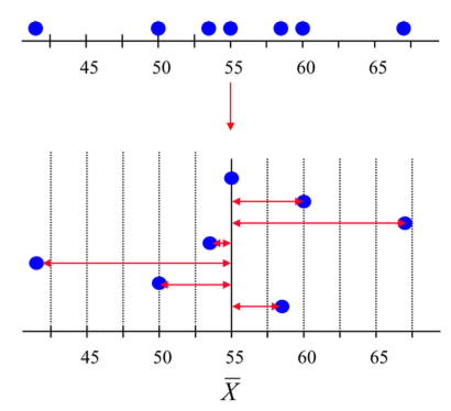
As its name suggests, the standard deviation tells what is the “normal” deviation of the data. It actually computes the mean deviation from the global mean. The larger the standard deviation, the more scattered the data are. On the contrary, the smaller the standard deviation, the more the data are centered around the mean. Below a visual representation of the standard deviation:
The standard deviation is a bit more complex than the previous statistics in the sense that there are two formulas depending on whether we face a sample or a population. A population includes all members from a specified group, all possible outcomes or measurements that are of interest. A sample consists of some observations drawn from the population, so a part or a subset of the population. For instance, the population may be “all people living in Belgium” and the sample may be “some people living in Belgium”. Read this article on the difference between population and sample if you want to learn more.
Standard deviation for a population
The standard deviation for a population, denoted \(\sigma\), is:
\[\sigma = \sqrt{\frac{1}{n}\sum^n_{i = 1}(x_i - \mu)^2}\]
As you can see from the formula, the standard deviation is actually the mean deviation of the data from the global mean \(\mu\). Note the square for the difference between the observations (\(x_i\)) and the mean (\(\mu\)) to avoid that negative differences are compensated by positive differences.
For the sake of easiness, imagine a population of only 3 adults (the steps are the same with a large population, the computation is just longer). Below their heights (in cm):
160.4, 175.8 and 181.5
The mean is 172.6 (rounded to 1 decimal). The standard deviation is thus:
\[\sigma = \sqrt{\frac{1}{3} \big[(160.4 - 172.6)^2 \\ + (175.8 - 172.6)^2 \\ + (181.5 - 172.6)^2 \big]}\] \[\sigma = 8.91\]
In conclusion, the standard deviation for the heights of these 3 adults is 8.91 cm. This means that, on average, the height of the adults in this population deviates from the mean by 8.91 cm.
Standard deviation for a sample
The standard deviation for a sample is similar to the standard deviation for a population except that we divide by \(n -1\) instead of \(n\) and it is denoted \(s\):
\[s = \sqrt{\frac{1}{n-1}\sum^n_{i = 1}(x_i - \bar{x})^2}\]
Imagine now that the 3 adults presented in the previous section is a sample instead of a population:
160.4, 175.8 and 181.5
The mean is still 172.6 (rounded to 1 decimal) since the mean is the same whether it is a population or a sample. The standard deviation is now:
\[s = \sqrt{\frac{1}{3 - 1} \big[(160.4 - 172.6)^2 \\ + (175.8 - 172.6)^2 \\ + (181.5 - 172.6)^2 \big]}\] \[s = 10.92\]
In conclusion, the standard deviation for the heights of these 3 adults is 10.92 cm. The interpretation is the same than for a population.
Variance
The variance is simply the square of the standard deviation. Put it another way, the standard deviation is the square root of the variance. We also distinguish between the variance for a population and for a sample in the next sections.
Variance for a population
The variance for a population, denoted \(\sigma^2\), is:
\[\sigma^2 = \frac{1}{n}\sum^n_{i = 1}(x_i - \mu)^2\]
As you can see, the formula for variance is the same than for standard deviation, except that the square root is removed for the variance. Remember the heights of our population of 3 adults:
160.4, 175.8 and 181.5
The standard deviation was 8.91 cm, so the variance of the height of these adults is \(8.91^2 = 79.39\) \(cm^2\) (see below why the unit of a variance is \(unit^2\)).
If you did not know the standard deviation of the population and needed to compute the variance of the population by hand, here is how:
\[\sigma^2 = \frac{1}{3} \big[(160.4 - 172.6)^2 \\ + (175.8 - 172.6)^2 \\ + (181.5 - 172.6)^2 \big] \\ = 79.43\]
(The difference with the above result is due to rounding.)
Variance for a sample
Again, the variance for a sample is similar to the variance for a population except that we divide by \(n - 1\) instead of \(n\) and it is denoted \(s^2\):
\[s^2 = \frac{1}{n-1}\sum^n_{i = 1}(x_i - \bar{x})^2\]
Imagine again that the 3 adults in the previous section is a sample instead of a population:
160.4, 175.8 and 181.5
The standard deviation for this sample was 10.92 cm, so the variance of the height of these adults is \(10.92^2 = 119.25\) \(cm^2\).
If you did not know the standard deviation of the sample and needed to compute the variance of the sample by hand, here is how:
\[s^2 = \frac{1}{3 - 1} \big[(160.4 - 172.6)^2 \\ + (175.8 - 172.6)^2 \\ + (181.5 - 172.6)^2 \big] \\ = 119.15\]
(The difference with the above result is due to rounding.)
Standard deviation vs. variance
Standard deviation and variance are often used interchangeably and both quantify the spread of a given dataset by measuring how far the observations are from their mean. However, the standard deviation can be more easily interpreted because the unit for the standard deviation is the same than the unit of measurement of the data (while it is the \(unit^2\) for the variance).
Following our example of adult heights in cm, the standard deviation is measured in cm while the variance is measured in \(cm^2\). The fact that the standard deviation keeps the same unit than the initial unit of measurement makes it more interpretable and thus more often used in practice.
Notations
For completeness, below a table showing the different notations for variance and standard deviation in case of population and sample:
| Population | Sample | |
|---|---|---|
| Standard deviation | \(\sigma\) | \(s\) |
| Variance | \(\sigma^2\) | \(s^2\) |
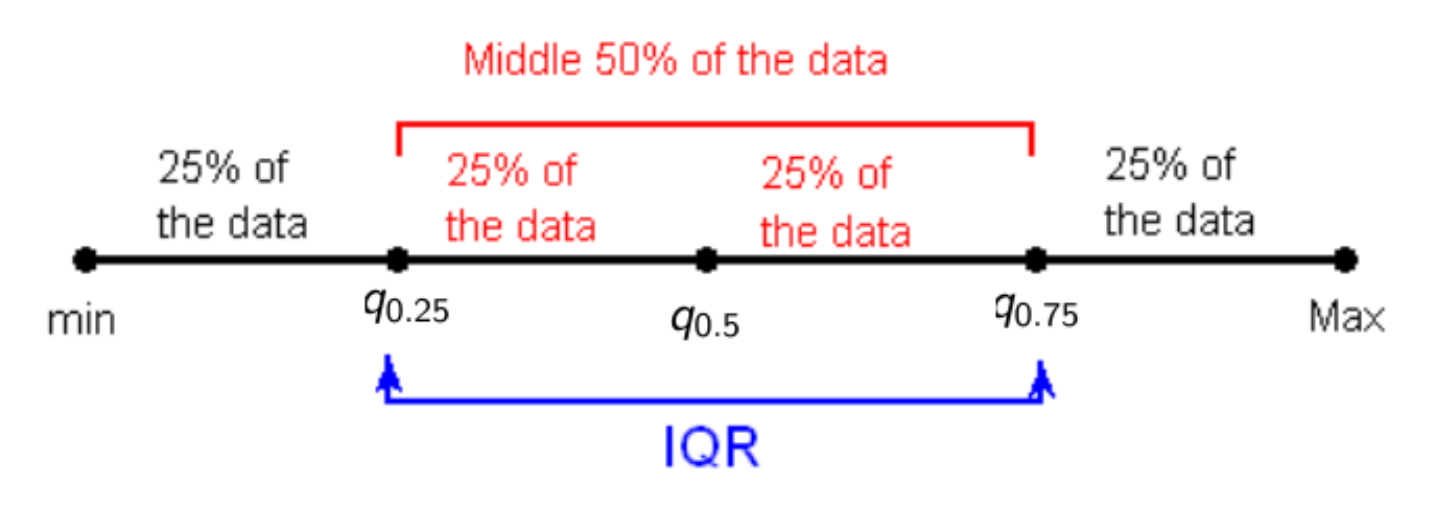
Interquartile range
Remember the first \(q_{0.25}\) and third quartile \(q_{0.75}\) presented earlier (see this section). The interquartile range is another measure of dispersion of the data, using the quartiles. It is the difference between the third and first quartile:
\[IQR = q_{0.75} - q_{0.25}\]
Considering the height of the 9 adults presented in the section about the first and third quartile:
170.2, 181.5, 188.9, 163.9, 166.4, 163.7, 160.4, 175.8 and 181.5
The first quartile was 163.9 cm and the third quartile was 181.5 cm. The IQR is thus:
\[IQR = 181.5 - 163.9 = 17.6\]
In conclusion, the interquartile range is 17.6 cm. The interquartile range is actually the range (since it is the difference between a higher and a lower value) of the middle data. The graph below may help to understand better the IQR and the quartiles:
Coefficient of variation
The last dispersion measure is the coefficient of variation. The coefficient of variation, denoted \(CV\), is the standard deviation divided by the mean. Formally:
\[CV = \frac{s}{\bar{x}}\]
Consider the height of a sample of 4 adults:
163.7, 160.4, 175.8 and 181.5
The mean is \(\bar{x} =\) 170.35 cm and the standard deviation is \(s =\) 9.95 cm. (Find the same values as an exercise!) The coefficient of variation is
\[CV = \frac{9.95 \text{ cm}}{170.35 \text{ cm}} = 0.058 = 5.8\%\]
In conclusion, the coefficient of variation is 5.8%. Note that, as a rule of thumb, a coefficient of variation greater than 15% usually means that the data are heterogeneous while a coefficient of variation equal to or less than 15% means that the data are homogeneous. Given that the coefficient of variation equals 5.8% in this case, we can conclude that these 4 adults are homogeneous in terms of height.
Note that the coefficient of variation for a population follows the same formula, except that notations for the mean and the standard deviation differ:
\[CV = \frac{\sigma}{\mu}\]
The interpretation is also the same as for a sample.
Coefficient of variation vs. standard deviation
Although the coefficient of variation is rather unknown to the public, it is, in fact, worth presenting when making descriptive statistics.
The standard deviation should always be understood in the context of the mean of the data and is dependent on its unit. The standard deviation has the advantage that it tells by how far on average the data is from the mean in terms of unit in which the data has been measured. Standard deviation is useful when considering variables with same units and approximately same means. However, standard deviation becomes less useful when comparing variables with different units or widely different means. For instance, a variable with a standard deviation of 10 cm cannot be compared to a variable with a standard deviation of 12€ to conclude which one of the two is the most dispersed.
The coefficient of variation is a ratio of two statistics with the same units. It has thus no unit and is independent of the unit in which the data has been measured. Being unit-free, coefficients of variation computed on datasets or variables with different units or widely different means can be compared to conclude, in fine, which data or variables is more (or less) dispersed. For instance, consider a sample of 10 women with their heights in cm and their salaries in €. We cannot compare the dispersion of their weights with the dispersion of their salaries because it is not measured on the same unit/scale. Now suppose that the coefficients of variation are 0.032 and 0.061 respectively for the height and the salary. Based on that, we can conclude that, relative to their respective average, their salaries vary more than their heights for these women. This is the case because the coefficient of variation is larger for the salary compared to the coefficient variation for the height, and a coefficient of variation has no unit (it is a ratio).
Conclusion
Remember that descriptive statistics are useful to describe and present a series of observations in a concise and informative way. There are two families of descriptive statistics: location and dispersion measures. Location measures give information about the position of the data, whereas dispersion measures give information about the variability of the data.
We showed how to compute the most common descriptive statistics by hand with concrete examples. We also discussed differences between some measures and when it is more appropriate to use one or the other depending on the context and the data at hand.
This concludes a relatively long article, thanks for reading! If you would like to learn how to compute these measures in R, read the article “Descriptive statistics in R”. A book I recommend for further reading is “The Art of Statistics” by David Spiegelhalter. It is a great book for beginners in statistics and covers a wide range of topics.
As always, if you have a question or a suggestion related to the topic covered in this article, please add it as a comment so other readers can benefit from the discussion.
This image and the following ones are taken from the LFSAB1105 course syllabus at UCLouvain.↩︎
Liked this post?
- Get updates every time a new article is published (no spam and unsubscribe anytime)
- Support the blog
- Share on:


