
Pearson, Spearman and Kendall correlation coefficients by hand

Introduction
In statistics, a correlation is used to evaluate the relationship between two variables.
In a previous post, we showed how to compute a correlation and perform a correlation test in R. In this post, we illustrate how to compute the Pearson, Spearman and Kendall correlation coefficients by hand and under two different scenarios (i.e., with and without ties).
Data
To illustrate the methods with and without ties, we consider two different datasets, one with ties and another without ties.
With ties
For the illustrations of the scenarios with ties, suppose we have the following sample of size 5:
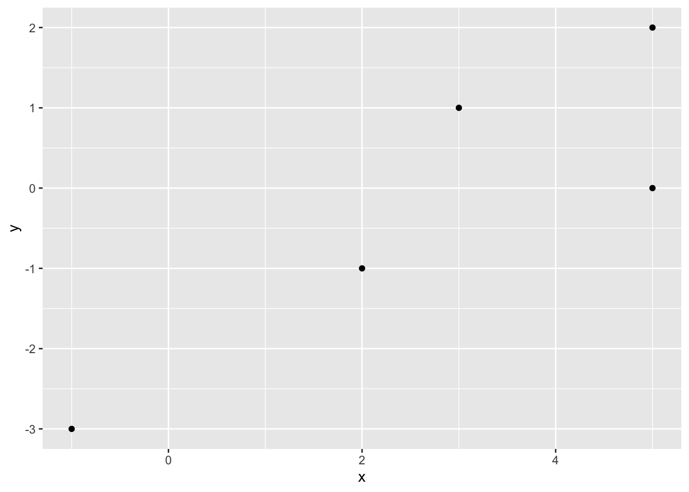
As we can see, there are some ties since there are two identical observations in the variable \(x\).
Without ties
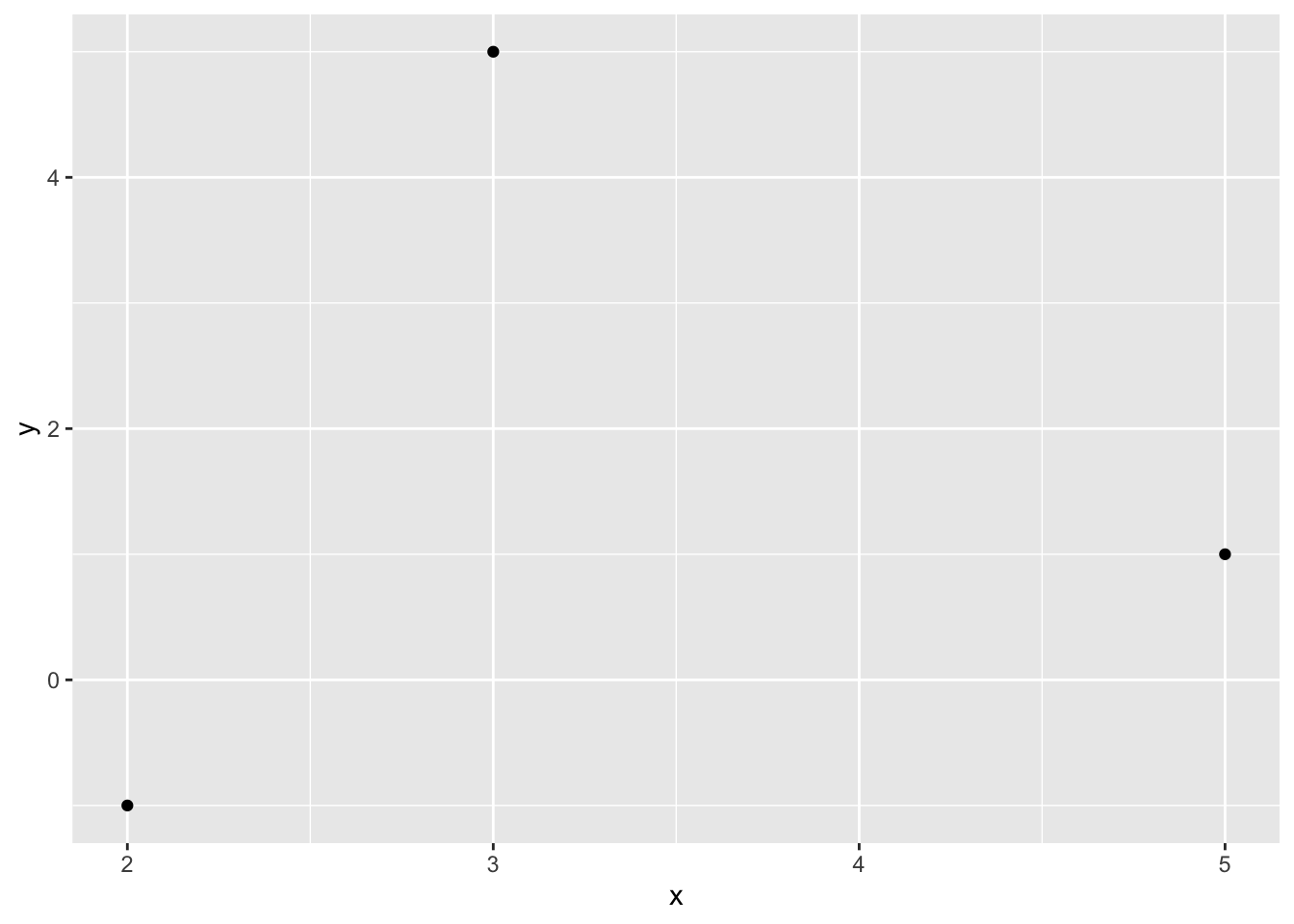
For the scenarios which require no ties, we will consider the following sample of size 3:
Correlation coefficients by hand
The three most common correlation methods are:1
- Pearson, used for two quantitative continuous variables which have a linear relationship
- Spearman, used for two quantitative variables if the link is partially linear, or for one qualitative ordinal variable and one quantitative variable
- Kendall, often used for two qualitative ordinal variables
Each method is presented in the next sections.
Note that the aim of this post is to illustrate how to compute the three correlation coefficients by hand and under two different scenarios; we are not interested in verifying the underlying assumptions.
Pearson
Luckily, the procedure for computing the Pearson correlation coefficient is the same whether there are ties or not so we do not distinguish the two scenarios.
With and without ties
The Pearson correlation coefficient, denoted \(r\) in the case of a sample, can be computed as follows2
\[ r = \frac{\sum^n_{i = 1} x_i y_i - n \bar{x} \bar{y}}{(n - 1) s_x s_y} \]
where:
- \(n\) is the sample size
- \(x_i\) and \(y_i\) are the observations
- \(\bar{x}\) and \(\bar{y}\) are the sample means of \(x\) and \(y\)
- \(s_x\) and \(s_y\) are the sample standard deviations of \(x\) and \(y\)
We show how to compute it step by step.
Step 1.
As you can see, before computing the correlation coefficient we first need to compute the mean and the standard deviation for each of the two variables.
The mean of \(x\) is computed as follows:
\[\bar{x} = \frac{1}{n}\sum^n_{i = 1} x_i\]
The standard deviation of \(x\) is computed as follows:
\[s_x = \sqrt{\frac{1}{n - 1} \sum^n_{i = 1}(x_i - \bar{x})^2}\]
The formulas can be used analogously for the variable \(y\).
We start by computing the means of the two variables:
- \(\bar{x} = \frac{-1 + 3 + 5 + 5 + 2}{5} = 2.8\)
- \(\bar{y} = \frac{-3 + 1 + 0 + 2 - 1}{5} = -0.2\)
Step 2.
We now need to compute the standard deviation of each variable. To ease the computations, it is best to use a table, starting with the observations:
To compute the standard deviations, we need the sum of the squared differences between each observation and its mean, that is, \(\sum^n_{i = 1}(x_i - \bar{x})^2\) and \(\sum^n_{i = 1}(y_i - \bar{y})^2\). We start by creating two new columns in the table, denoted x-xbar and y-ybar, corresponding to \((x_i - \bar{x})\) and \((y_i - \bar{y})\):
We take the square of these two new columns to have \((x_i - \bar{x})^2\) and \((y_i - \bar{y})^2\), denoted (x-xbar)^2 and (y-ybar)^2:
We then sum these two columns, which gives:
- for \(x\): \(\sum^n_{i = 1}(x_i - \bar{x})^2 =\) 24.8
- for \(y\): \(\sum^n_{i = 1}(y_i - \bar{y})^2 =\) 14.8
The standard deviations are thus:
- \(s_x = \sqrt{\frac{24.8}{5-1}} = 2.49\)
- \(s_y = \sqrt{\frac{14.8}{5-1}} = 1.92\)
Step 3.
We now need \(\sum^n_{i = 1} x_i y_i\), so we add a new column in the table, corresponding to \(x_iy_i\) and denoted x*y:
Step 4.
We take the sum of that last column, which gives \(\sum^n_{i = 1} x_i y_i =\) 14.
Step 5.
Finally, the Pearson correlation coefficient can be computed by plugging values found above in the initial formula:
\[ \begin{split} r &= \frac{\sum^n_{i = 1} x_i y_i - n \bar{x} \bar{y}}{(n - 1) s_x s_y} \\ &= \frac{14 - (5\times2.8\times-0.2)}{(5-1) \times 2.49\times1.92} \\ &= 0.88 \end{split} \]
Note that there are other formulas to compute the Pearson correlation coefficient. For instance,
\[ \begin{split} r &= \frac{1}{n - 1} \sum^n_{i = 1} \left(\frac{x_i - \bar{x}}{s_x}\right)\left(\frac{y_i - \bar{x}}{s_y}\right) \\ &= \frac{\sum^n_{i = 1}(x_i - \bar{x})(y_i - \bar{y})}{\sqrt{\sum^n_{i = 1}(x_i - \bar{x})^2} \sqrt{\sum^n_{i = 1}(y_i - \bar{y})^2}} \end{split} \]
All formulas will of course give the exact same results.
For your information, squaring the Pearson correlation coefficient \(r\) gives the coefficient of determination \(R^2\) in the context of a simple linear regression.
Spearman
We now present the Spearman correlation coefficient, also referred as Spearman’s rank correlation coefficient. This coefficient is actually the same than Pearson coefficient, except that the computations are based on the ranked values rather than on the raw observations.
Again, we present how to compute it by hand step by step, but this time we distinguish two scenarios:
- if there are ties
- if there are no ties
With ties
The Spearman correlation coefficient (with ties), denoted \(r_s\), is defined as follows
\[ r_s = \frac{\sum^n_{i = 1} Rx_i Ry_i - n \overline{Rx} \overline{Ry}}{(n - 1) s_{Rx} s_{Ry}} \]
where:
- \(n\) is the sample size
- \(Rx_i\) and \(Ry_i\) are the ranks for the two variables
- \(\overline{Rx}\) and \(\overline{Ry}\) are the sample means of the ranks for the two variables
- \(s_{Rx}\) and \(s_{Ry}\) are the sample standard deviations of the ranks for the two variables
Here is how to compute it by hand.
Step 1.
As mentioned before, the Spearman coefficient is based on the ranks. So we first need to add the ranks of the observations (from lowest to highest), separately for each of the two variables.
For \(y\), we see that:
- -3 is the smallest value, so we assign it the rank 1
- -1 is the second smallest value, so we assign it the rank 2
- then comes 0, so we assign it the rank 3
- then comes 1, so we assign it the rank 4
- finally, 2 is the largest value, so we assign it the rank 5
The same goes for \(x\), except that here we have two observations with the value 5 (so there will be ties in the ranks). In this case, we take the mean rank:
- -1 is the smallest value, so we assign it the rank 1
- 2 is the second smallest value, so we assign it the rank 2
- then comes 3, so we assign it the rank 3
- finally, the two largest values belongs to rank 4 and 5, so we assign both of them the rank 4.5
We include the ranks in the table, denoted Rx and Ry:
Step 2.
From there, it is similar than the Pearson coefficient except that we work on the ranks and not on the initial observations anymore. To avoid any confusion in the remaining steps, we remove the initial observations from the table and we keep only the ranks:
We start with the means of the ranks:
- \(\overline{Rx} = \frac{1+3+4.5+4.5+2}{5} = 3\)
- \(\overline{Ry} = \frac{1+4+3+5+2}{5} = 3\)
For the standard deviations, we use the table as we did for the Pearson coefficient:
We sum the last two columns, which gives:
- for \(x\): \(\sum^n_{i = 1}(Rx_i - \overline{Rx})^2 =\) 9.5
- for \(y\): \(\sum^n_{i = 1}(Ry_i - \overline{Ry})^2 =\) 10
The standard deviations are thus:
- \(s_{Rx} = \sqrt{\frac{9.5}{5-1}} = 1.54\)
- \(s_{Ry} = \sqrt{\frac{10}{5-1}} = 1.58\)
Step 3.
We now need \(\sum^n_{i = 1} Rx_i Ry_i\), so we add a new column in the table, corresponding to \(Rx_iRy_i\) and denoted Rx*Ry:
Step 4.
We take the sum of that last column, which gives \(\sum^n_{i = 1} Rx_i Ry_i =\) 53.
Step 5.
Finally, the Spearman correlation coefficient can be computed by plugging all values in the initial formula:
\[ \begin{split} r_s &= \frac{\sum^n_{i = 1} Rx_i Ry_i - n \overline{Rx} \overline{Ry}}{(n - 1) s_{Rx} s_{Ry}} \\ &= \frac{53 - (5\times3\times3)}{(5-1) \times 1.54\times1.58} \\ &= 0.82 \end{split} \]
Without ties
When all initial values are different within each variable, meaning that all ranks are distinct integers, there are no ties. In that specific case, the Spearman coefficient can be computed with the following shortened formula:
\[ r_s = 1 - \frac{6 \sum^n_{i = 1}(Rx_i - Ry_i)^2}{n (n^2 - 1)} \]
For example, suppose the sample without ties introduced at the beginning of the post:
Step 1.
All observations within each variable are different, so all ranks are distinct integers and there are no ties:
Step 2.
We only need to compute the difference between the two ranks of each row, denoted Rx-Ry:
Take the square of these differences, denoted (Rx-Ry)^2:
And then take the sum of that last column, which gives \(\sum^n_{i = 1}(Rx_i - Ry_i)^2 =\) 2.
Step 3.
Finally, we can fill in the initial formula to find the Spearman coefficient:
\[ \begin{split} r_s &= 1 - \frac{6 \sum^n_{i = 1}(Rx_i - Ry_i)^2}{n (n^2 - 1)} \\ &= 1 - \frac{6 \times2}{3 (3^2 - 1)} \\ &= 1 - \frac{12}{24} \\ &= 0.5 \end{split} \]
Kendall
Kendall coefficient correlation, also known as Kendall’s \(\tau\) coefficient, is similar than Spearman coefficient, except that it is often preferred for small samples and when many rank ties.
Here also we distinguish between two scenarios:
- if there are no ties
- if there are ties
Unlike Spearman coefficient, we first illustrate the scenario when there are no ties, and then when there are ties.
Without ties
When there are no ties, the Kendall coefficient, denoted \(\tau_a\), is defined as follows
\[ \tau_a = \frac{C - D}{C + D} \]
where:
- \(C\) is the number of concordant pairs
- \(D\) is the number of discordant pairs
This coefficient, also referred as Kendall tau-a, does not make any adjustment for ties.
Let’s see what are concordant and discordant pairs using the data without ties (the same data than for Spearman correlation without ties):
Step 1.
We start by computing the ranks for each variable (Rx and Ry), as we did for the Spearman coefficient:
Step 2.
We then arbitrarily choose a reference variable among the two, Rx or Ry. Suppose we take Rx as the reference variable here.
We sort the dataset by this reference variable:
From now, we only look at the ranks of the second variable (the one which is not the reference level, here Ry), so to avoid any confusion in the remaining steps we keep only the Ry column:
Step 3.
We now take each row of Ry one by one and check whether the rows below it in the table are smaller or larger.
In our table, the first row of Ry is 1. We see that the value just below it is 3, which is larger than 1. Since 3 is larger than 1, this is called a concordant pair. We write it in the table:
The next row, 2, is also larger than 1, so it is also a concordant pair. We also write it in the table:
We start again with the second row of Ry, which is 3. Again, we look at the row below it and check whether it is larger or smaller. Here, the row below it is 2, which is smaller than 3, so we have a discordant pair. We add this information into the table:
Step 4.
We now compute the total number of concordant and discordant pairs. There are:
- 2 concordant pairs so \(C = 2\), and
- 1 discordant pair so \(D = 1\).
Step 5.
Finally, we plug the values we have just found in the initial formula:
\[ \begin{split} \tau_a &= \frac{C - D}{C + D}\\ &= \frac{2 - 1}{2 + 1}\\ &= \frac{1}{3}\\ &= 0.33 \end{split} \]
Alternatively, we can also use the following formulas
\[ \begin{split} \tau_a &= 1 - \frac{4D}{n(n - 1)}\\ &= \frac{4C}{n(n - 1)} - 1 \end{split} \]
where \(n\) is still the sample size, and which both give the exact same results.
With ties
I must admit that the process with ties is slightly more complex than without ties.
The Kendall tau-b coefficient, which makes adjustments for ties, is defined as follows
\[ \tau_b = \frac{C - D}{\sqrt{(C^2_n - n_x)(C^2_n - n_y)}} \]
where:
- \(C\) and \(D\) are still the number of concordant and discordant pairs, respectively
- \(C^2_n\) is the total number of possible pairs
- \(n_x\) is the number of possible pairs with a tie among the \(x\) values
- \(n_y\) is the number of possible pairs with a tie among the \(y\) values
Note that here, the letter \(C\) in \(C^2_n\) denotes “combination” and not “concordant”.
Let’s illustrate that scenario and the formula with the dataset used for the Pearson correlation and the Spearman correlation with ties, that is:
Step 1.
Similarly to with no ties, the process with ties is based on the ranks so we start by adding the ranks for each variable, denoted as usual as Rx and Ry:
Step 2.
One of the two variables (\(x\) or \(y\)) must be selected as the reference variable. This time, we do not choose it arbitrarily, but we choose the one which does not have any ties. In our case, variable \(x\) has ties, while variable \(y\) does not have any ties. So \(y\) will be our reference variable.
We then:
- order the dataset by the reference variable, here
Ry, and - we keep only the necessary columns to avoid any confusion in the remaining steps:
Step 3.
We check whether it is a concordant or discordant pair the same way we did without ties, but this time we do not count ties.
The first row in column Rx is 1. We compare all rows below it in the table with that value. All rows below 1 in the table are larger, so we write that they are concordant pairs:
We repeat the same process for each row.
For instance, for the second row of the column Rx, we have the value 2. Again, all rows below in the table are larger so we write that they are concordant pairs:
For the third row of the column Rx, we have the value 4.5. The row just below in the table (= 3) is smaller than 4, so we write D for discordant pair:
Now, as you can see, the last row is also 4.5. Therefore, since it is equal to the value we are comparing to, it is neither a concordant nor a discordant pair, so we write “T” in the table for “ties”:
Last, the fourth row in the column Rx is 3, which we compare to 4.5 to see that 4.5 is larger so it is a concordant pair:
Step 4.
We then sum the number of concordant and discordant pairs:
- \(C = 8\)
- \(D = 1\)
Step 5.
We now have all the information required to compute the numerator of \(\tau_b\), but we still need to find \(C^2_n\), \(n_x\) and \(n_y\) to compute the denominator.
As mentioned above, \(C^2_n\) is the total number of possible pairs, thus corresponding to the number of combinations of two values. This number of pairs can be found with the formula of the combination, that is, \(C^2_n = \frac{n!}{2!(n - 2)!}\) where \(n\) is the sample size.
In our case, we have a sample of size 5, so we have:3
\[ \begin{split} C^2_n &= \frac{n!}{2!(n - 2)!}\\ &= \frac{5!}{2!(5-2)!}\\ &= 10 \end{split} \]
Furthermore, \(n_x\) and \(n_y\) are the number of possible pairs with a tie among the \(x\) and \(y\) variables, respectively.
When looking at Ry and Rx from the table above:
We see that there are:
- 2 identical values for the variable \(x\)
- 0 identical value for the variable \(y\)
This means that the number of possible pairs with a tie is equal to:4
- 1 for the variable \(x\) (the only possible pair with a tie is the pair {4.5, 4.5})
- 0 for the variable \(y\) (since all ranks are distinct, there exists no pair with a tie)
Therefore,
\[ \begin{split} n_x &= 1\\ n_y &= 0 \end{split} \]
And we now have all the necessary information to compute \(\tau_b\)!
Step 6.
By plugging the values found above in the initial formula, we have
\[ \begin{split} \tau_b &= \frac{C - D}{\sqrt{(C^2_n - n_x)(C^2_n - n_y)}}\\ &= \frac{8-1}{\sqrt{(10 - 1)(10 - 0)}}\\ &= \frac{7}{\sqrt{90}}\\ &= 0.74 \end{split} \]
Verification in R
For the sake of completeness, we verify our results with the help of R for each coefficient and scenario.
Pearson:
x <- c(-1, 3, 5, 5, 2)
y <- c(-3, 1, 0, 2, -1)

cor(x, y, method = "pearson")
## [1] 0.8769051Spearman with ties:
cor(x, y, method = "spearman")## [1] 0.8207827Spearman without ties:
x2 <- c(3, 5, 2)
y2 <- c(5, 1, -1)

cor(x2, y2, method = "spearman")
## [1] 0.5Kendall without ties:
cor(x2, y2, method = "kendall")## [1] 0.3333333Kendall with ties:
cor(x, y, method = "kendall")## [1] 0.7378648We indeed find the same results by hand than with R (any discrepancies is due to rounding)!
Conclusion
Remember that a correlation coefficient (no matter whether it is Pearson, Spearman or Kendall) ranges from -1 to 1, with 0 being no correlation and the closer to 1 in absolute terms, the stronger the correlation.
Broadly speaking, a positive correlation means that high values of one variable are associated with high values of the other variable (and vice versa). A negative correlation means that high values of one variable are associated with low values of the other variable.
Last but not least, remember that the conclusions drawn from a correlation coefficient computed within a sample cannot be generalized to the population without a proper statistical test, that is, a correlation test.
Thanks for reading.
I hope this article helped you to compute the Pearson, Spearman and Kendall correlation coefficients by hand (with and without ties).
As always, if you have a question or a suggestion related to the topic covered in this article, please add it as a comment so other readers can benefit from the discussion.
For your information, the Pearson correlation coefficient is considered as a parametric procedure, whereas the Spearman and Kendall correlation coefficients are considered as non-parametric procedures.↩︎
Here, we suppose that we have a sample and not a population. In the case where the observations you have represent the entire population, the correlation coefficient is denoted \(\rho\) and the formula differs slightly. See a recap of the difference between a sample and a population if needed.↩︎
Remember that the factorial of \(n\), denoted \(n!\), is \(n! = n \times (n - 1) \times \cdots \times 1\). So for instance, \(5! = 5\times4\times3\times2\times1 = 120\).↩︎
If you have many identical values and want to count the number of possible pairs thanks to a formula rather than by counting them manually, you can again use the formula of the combination, that is, \(C^2_n = \frac{n!}{x!(n - x)!}\) where \(n\) is the number of identical values in a given group of ties. Bear in mind that the number of combinations must be summed up for all group of ties. In our case, we have only one group of ties with 2 values, so \(n_x = C^2_2 = \frac{2!}{2!(2 - 2)!} = 1\).↩︎
Liked this post?
- Get updates every time a new article is published (no spam and unsubscribe anytime)
- Support the blog
- Share on:


