
Tips and tricks in RStudio and R Markdown
- Run code
- Insert a comment in R and R Markdown
- Knit a R Markdown document
- Code snippets
- Ordered list in R Markdown
- New code chunk in R Markdown
- Reformat code
- RStudio addins
{pander}and{report}for aesthetics- Extract equation model with
{equatiomatic} - Print model’s parameters
- Pipe operator
%>% - Others
- Conclusion
If you have the chance to work with an experienced programmer, you may be amazed by how fast she can write code. In this article, I share some tips and shortcuts you can use in RStudio and R Markdown to speed up the writing of your code.
Run code
You most probably already know this shortcut but I still mention it for new R users. From your script you can run a chunk of code with:
command + Enter on Mac
Ctrl + Enter on Windows
Insert a comment in R and R Markdown
To insert a comment:
command + Shift + C on Mac
Ctrl + Shift + C on Windows
This shortcut can be used both for:
- R code when you want to comment your code. It will add a
#at the beginning of the line - for text in R Markdown. It will add
<!--and-->around the text
Note that if you want to comment more than one line, select all the lines you want to comment then use the shortcut. If you want to uncomment a comment, apply the same shortcut.
Knit a R Markdown document
You can knit R Markdown documents by using this shortcut:
command + Shift + K on Mac
Ctrl + Shift + K on Windows
Code snippets
Code snippets is usually a few characters long and is used as a shortcut to insert a common piece of code. You simply type a few characters then press Tab and it will complete your code with a larger code. Tab is then used again to navigate through the code where customization is required. For instance, if you type fun then press Tab, it will auto-complete the code with the required code to create a function:
name <- function(variables) {

}
Pressing Tab again will jump through the placeholders for you to edit it. So you can first edit the name of the function, then the variables and finally the code inside the function (try by yourself!).
There are many code snippets by default in RStudio. Here are the code snippets I use most often:
libto calllibrary()
library(package)matto create a matrix
matrix(data, nrow = rows, ncol = cols)if,el, andeito create conditional expressions such asif() {},else {}andelse if () {}
if (condition) {

}

else {

}

else if (condition) {

}funto create a function
name <- function(variables) {

}forto create for loops
for (variable in vector) {

}tsto insert a comment with the current date and time (useful if you have very long code and share it with others so they see when it has been edited)
# Tue Jan 21 20:20:14 2020 ------------------------------shinyappevery time I create a new shiny app
library(shiny)

ui <- fluidPage()

server <- function(input, output, session) {

}

shinyApp(ui, server)
You can see all default code snippets and add yours by clicking on Tools > Global Options… > Code (left sidebar) > Edit Snippets…
Ordered list in R Markdown
In R Markdown, when creating an ordered list such as this one:
- Item 1
- Item 2
- Item 3
Instead of bothering with the numbers and typing
1. Item 1
2. Item 2
3. Item 3
you can simply type
1. Item 1
1. Item 2
1. Item 3
for the exact same result (try it yourself or check the code of this article!). This way you do not need to bother which number is next when creating a new item.
To go even further, any numeric will actually render the same result as long as the first item is the number you want to start from. For example, you could type:
1. Item 1
7. Item 2
3. Item 3
which renders
- Item 1
- Item 2
- Item 3
However, I suggest always using the number you want to start from for all items because if you move one item at the top, the list will start with this new number. For instance, if we move 7. Item 2 from the previous list at the top, the list becomes:
7. Item 2
1. Item 1
3. Item 3
which incorrectly renders
- Item 2
- Item 1
- Item 3
New code chunk in R Markdown
When editing R Markdown documents, you will need to insert a new R code chunk many times. The following shortcuts will make your life easier:
command + option + I on Mac (or command + alt + I depending on your keyboard)
Ctrl + ALT + I on Windows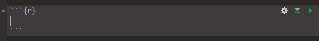
New R code chunk in R Markdown
Reformat code
A clear and readable code is always easier and faster to read (and look more professional when sharing it to collaborators). To automatically apply the most common coding guidelines such as whitespaces, indents, etc., use:
cmd + Shift + A on Mac
Ctrl + Shift + A on Windows
So for example the following code which does not respect the guidelines (and which is not easy to read):
1+1
  for(i in 1:10){if(!i%%2){next}
print(i)
 }
becomes much more neat and readable:
1 + 1
for (i in 1:10) {
  if (!i %% 2) {
    next
  }
  print(i)
}
RStudio addins
RStudio addins are extensions which provide a simple mechanism for executing advanced R functions from within RStudio. In simpler words, when executing an addin (by clicking a button in the Addins menu), the corresponding code is executed without you having to write the code. RStudio addins have the advantage that they allow you to execute complex and advanced code much more easily than if you would have to write it yourself.
The addin I use most often is probably the {esquisse} addin, which allows to draw plots with the {ggplot2} package in a user-friendly and interactive way, and without having to write the code myself.
RStudio addins are quite diverse and require a more detailed explanation, so I wrote an article focusing on these addins. See the article here.
{pander} and {report} for aesthetics
The pander() function from the {pander} package is very useful for R Markdown documents and reporting. It is not actually a shortcut but it greatly improves the aesthetics of R outputs.
For instance, see below the difference between the default output of a Chi-square test of independence and the output from the same test with the pander() function (using the diamonds dataset from the {ggplot2} package):
library(ggplot2)
dat <- diamonds

test <- chisq.test(table(dat$cut, dat$color))
test
##
## Pearson's Chi-squared test
##
## data: table(dat$cut, dat$color)
## X-squared = 310.32, df = 24, p-value < 2.2e-16library(pander)
pander(test)| Test statistic | df | P value |
|---|---|---|
| 310.3 | 24 | 1.395e-51 * * * |
All information that you need are displayed in an elegant table. The pander() function works on many statistical tests (not to say all of them, but I have not tried it on all available tests in R) and on regression models:
# Linear model with lm()
model <- lm(price ~ carat + x + y + z,
  data = dat
)
model
##
## Call:
## lm(formula = price ~ carat + x + y + z, data = dat)
##
## Coefficients:
## (Intercept) carat x y z
## 1921.2 10233.9 -884.2 166.0 -576.2pander(model)| Estimate | Std. Error | t value | Pr(>|t|) | |
|---|---|---|---|---|
| (Intercept) | 1921 | 104.4 | 18.41 | 1.977e-75 |
| carat | 10234 | 62.94 | 162.6 | 0 |
| x | -884.2 | 40.47 | -21.85 | 2.317e-105 |
| y | 166 | 25.86 | 6.421 | 1.365e-10 |
| z | -576.2 | 39.28 | -14.67 | 1.277e-48 |
The pander function also makes datasets, tables, vectors, etc. more readable in R Markdown output. For example, see the differences below:
head(dat)[1:7] # first 6 observations of the first 7 variables## # A tibble: 6 × 7
## carat cut color clarity depth table price
## <dbl> <ord> <ord> <ord> <dbl> <dbl> <int>
## 1 0.23 Ideal E SI2 61.5 55 326
## 2 0.21 Premium E SI1 59.8 61 326
## 3 0.23 Good E VS1 56.9 65 327
## 4 0.29 Premium I VS2 62.4 58 334
## 5 0.31 Good J SI2 63.3 58 335
## 6 0.24 Very Good J VVS2 62.8 57 336pander(head(dat)[1:7])| carat | cut | color | clarity | depth | table | price |
|---|---|---|---|---|---|---|
| 0.23 | Ideal | E | SI2 | 61.5 | 55 | 326 |
| 0.21 | Premium | E | SI1 | 59.8 | 61 | 326 |
| 0.23 | Good | E | VS1 | 56.9 | 65 | 327 |
| 0.29 | Premium | I | VS2 | 62.4 | 58 | 334 |
| 0.31 | Good | J | SI2 | 63.3 | 58 | 335 |
| 0.24 | Very Good | J | VVS2 | 62.8 | 57 | 336 |
summary(dat) # main descriptive statistics## carat cut color clarity depth
## Min. :0.2000 Fair : 1610 D: 6775 SI1 :13065 Min. :43.00
## 1st Qu.:0.4000 Good : 4906 E: 9797 VS2 :12258 1st Qu.:61.00
## Median :0.7000 Very Good:12082 F: 9542 SI2 : 9194 Median :61.80
## Mean :0.7979 Premium :13791 G:11292 VS1 : 8171 Mean :61.75
## 3rd Qu.:1.0400 Ideal :21551 H: 8304 VVS2 : 5066 3rd Qu.:62.50
## Max. :5.0100 I: 5422 VVS1 : 3655 Max. :79.00
## J: 2808 (Other): 2531
## table price x y
## Min. :43.00 Min. : 326 Min. : 0.000 Min. : 0.000
## 1st Qu.:56.00 1st Qu.: 950 1st Qu.: 4.710 1st Qu.: 4.720
## Median :57.00 Median : 2401 Median : 5.700 Median : 5.710
## Mean :57.46 Mean : 3933 Mean : 5.731 Mean : 5.735
## 3rd Qu.:59.00 3rd Qu.: 5324 3rd Qu.: 6.540 3rd Qu.: 6.540
## Max. :95.00 Max. :18823 Max. :10.740 Max. :58.900
##
## z
## Min. : 0.000
## 1st Qu.: 2.910
## Median : 3.530
## Mean : 3.539
## 3rd Qu.: 4.040
## Max. :31.800
## pander(summary(dat))| carat | cut | color | clarity | depth |
|---|---|---|---|---|
| Min. :0.2000 | Fair : 1610 | D: 6775 | SI1 :13065 | Min. :43.00 |
| 1st Qu.:0.4000 | Good : 4906 | E: 9797 | VS2 :12258 | 1st Qu.:61.00 |
| Median :0.7000 | Very Good:12082 | F: 9542 | SI2 : 9194 | Median :61.80 |
| Mean :0.7979 | Premium :13791 | G:11292 | VS1 : 8171 | Mean :61.75 |
| 3rd Qu.:1.0400 | Ideal :21551 | H: 8304 | VVS2 : 5066 | 3rd Qu.:62.50 |
| Max. :5.0100 | NA | I: 5422 | VVS1 : 3655 | Max. :79.00 |
| NA | NA | J: 2808 | (Other): 2531 | NA |
| table | price | x | y | z |
|---|---|---|---|---|
| Min. :43.00 | Min. : 326 | Min. : 0.000 | Min. : 0.000 | Min. : 0.000 |
| 1st Qu.:56.00 | 1st Qu.: 950 | 1st Qu.: 4.710 | 1st Qu.: 4.720 | 1st Qu.: 2.910 |
| Median :57.00 | Median : 2401 | Median : 5.700 | Median : 5.710 | Median : 3.530 |
| Mean :57.46 | Mean : 3933 | Mean : 5.731 | Mean : 5.735 | Mean : 3.539 |
| 3rd Qu.:59.00 | 3rd Qu.: 5324 | 3rd Qu.: 6.540 | 3rd Qu.: 6.540 | 3rd Qu.: 4.040 |
| Max. :95.00 | Max. :18823 | Max. :10.740 | Max. :58.900 | Max. :31.800 |
| NA | NA | NA | NA | NA |
table(dat$cut, dat$color) # contingency table##
## D E F G H I J
## Fair 163 224 312 314 303 175 119
## Good 662 933 909 871 702 522 307
## Very Good 1513 2400 2164 2299 1824 1204 678
## Premium 1603 2337 2331 2924 2360 1428 808
## Ideal 2834 3903 3826 4884 3115 2093 896pander(table(dat$cut, dat$color))| D | E | F | G | H | I | J | |
|---|---|---|---|---|---|---|---|
| Fair | 163 | 224 | 312 | 314 | 303 | 175 | 119 |
| Good | 662 | 933 | 909 | 871 | 702 | 522 | 307 |
| Very Good | 1513 | 2400 | 2164 | 2299 | 1824 | 1204 | 678 |
| Premium | 1603 | 2337 | 2331 | 2924 | 2360 | 1428 | 808 |
| Ideal | 2834 | 3903 | 3826 | 4884 | 3115 | 2093 | 896 |
names(dat) # variable names## [1] "carat" "cut" "color" "clarity" "depth" "table" "price"
## [8] "x" "y" "z"pander(names(dat))carat, cut, color, clarity, depth, table, price, x, y and z
rnorm(4) # generates 4 observations from a standard normal distribution## [1] 1.3709584 -0.5646982 0.3631284 0.6328626pander(rnorm(4))0.4043, -0.1061, 1.512 and -0.09466
This trick is particularly useful when writing in R Markdown, as the generated document will look much nicer.
Another trick for the aesthetics is the report() function from the {report} package.
Similar to pander(), the report() function allows to report test results in a more readable way—but it also interprets results for you. See for example with an ANOVA:
# install.packages("remotes")
# remotes::install_github("easystats/report") # You only need to do that once
library("report") # Load the package every time you start R

report(aov(price ~ cut,
  data = dat
))
## The ANOVA (formula: price ~ cut) suggests that:
##
## - The main effect of cut is statistically significant and small (F(4, 53935) =
## 175.69, p < .001; Eta2 = 0.01, 95% CI [0.01, 1.00])
##
## Effect sizes were labelled following Field's (2013) recommendations.In addition to the p-value and the test statistic, the result of the test is displayed and interpreted for you.
Note that the report() function can be used for other analyses. See more examples in the package’s documentation.
Extract equation model with {equatiomatic}
If you often need to write equations corresponding to statistical models in R Markdown reports, the {equatiomatic} will help you to save time.
Here is a basic example with a simple linear regression using the same dataset as above (i.e., diamonds from {ggplot2}):
# install.packages("equatiomatic")
library(equatiomatic)

# fit a basic multiple linear regression model
model <- lm(price ~ carat,
  data = dat
)

extract_eq(model,
  use_coefs = TRUE
)
\[ \operatorname{\widehat{price}} = -2256.36 + 7756.43(\operatorname{carat}) \]
If the equation is long, you can display it on multiple lines by adding the argument wrap = TRUE:
model <- lm(price ~ carat + x + y + z + depth,
  data = dat
)

extract_eq(model,
  use_coefs = TRUE,
  wrap = TRUE,
  terms_per_line = 2
)
\[ \begin{aligned} \operatorname{\widehat{price}} &= 12196.69 + 10615.5(\operatorname{carat})\ - \\ &\quad 1369.67(\operatorname{x}) + 97.6(\operatorname{y})\ + \\ &\quad 64.2(\operatorname{z}) - 156.62(\operatorname{depth}) \end{aligned} \]
Note that:
- If you use it in R Markdown, you need to add
results = 'asis'for that specific code chunk, otherwise the equation will be rendered as a LaTeX equation - At the time of writing, it works only for PDF and HTML output and not for Word
- The default number of terms per line is 4. You can change that with the
terms_per_lineargument {equatiomatic}supports output from logistic regression as well. See all supported models in the vignette- If you need the theoretical model without the actual parameter estimates, remove the
use_coefsargument:
extract_eq(model,
  wrap = TRUE
)
\[ \begin{aligned} \operatorname{price} &= \alpha + \beta_{1}(\operatorname{carat}) + \beta_{2}(\operatorname{x}) + \beta_{3}(\operatorname{y})\ + \\ &\quad \beta_{4}(\operatorname{z}) + \beta_{5}(\operatorname{depth}) + \epsilon \end{aligned} \]
In that case, I prefer to use \(\beta_0\) as intercept instead of \(\alpha\). You can change that with the intercept = "beta" argument:
extract_eq(model,
  wrap = TRUE,
  intercept = "beta"
)
\[ \begin{aligned} \operatorname{price} &= \beta_{0} + \beta_{1}(\operatorname{carat}) + \beta_{2}(\operatorname{x}) + \beta_{3}(\operatorname{y})\ + \\ &\quad \beta_{4}(\operatorname{z}) + \beta_{5}(\operatorname{depth}) + \epsilon \end{aligned} \]
Print model’s parameters
Thanks to the print_html() and model_parameters() functions from the {parameters} packages, you can print a summary of a model in a nicely formatted way to make the output more readable in your HTML file. See for instance with the multiple linear regression presented above:
library(parameters)
library(gt)

print_html(model_parameters(model, summary = TRUE))| Parameter | Coefficient | SE | 95% CI | t(53934) | p |
|---|---|---|---|---|---|
| (Intercept) | 12196.69 | 367.64 | (11476.10, 12917.27) | 33.18 | < .001 |
| carat | 10615.50 | 63.81 | (10490.43, 10740.56) | 166.37 | < .001 |
| x | -1369.67 | 43.48 | (-1454.89, -1284.45) | -31.50 | < .001 |
| y | 97.60 | 25.76 | (47.10, 148.10) | 3.79 | < .001 |
| z | 64.20 | 44.75 | (-23.51, 151.91) | 1.43 | 0.151 |
| depth | -156.62 | 5.38 | (-167.16, -146.09) | -29.13 | < .001 |
| Model: price ~ carat + x + y + z + depth (53940 Observations) Residual standard deviation: 1512.175 (df = 53934) R2: 0.856; adjusted R2: 0.856 |
|||||
Pipe operator %>%
If you are using the {dplyr}, {tidyverse} or {magrittr} packages often, here is a shortcut for the pipe operator %>%:
command + Shift + M on Mac
Ctrl + Shift + M on Windows
Others
Similar to many other programs, you can also use:
command + Shift + Non Mac andCtrl + Shift + Non Windows to open a new R Scriptcommand + Son Mac andCtrl + Son Windows to save your current script or R Markdown document
Conclusion
Thanks for reading.
I hope you find these tips and tricks useful. If you are using others, feel free to share them in the comment section. See this starting guide in R Markdown if you are not familiar with it.
As always, if you have a question or a suggestion related to the topic covered in this article, please add it as a comment so other readers can benefit from the discussion.
Liked this post?
- Get updates every time a new article is published (no spam and unsubscribe anytime)
- Support the blog
- Share on:


