Two-way ANOVA in R

Introduction
The two-way ANOVA (analysis of variance) is a statistical method that allows to evaluate the simultaneous effect of two categorical variables on a quantitative continuous variable.
The two-way ANOVA is an extension of the one-way ANOVA since it allows to evaluate the effects on a numerical response of two categorical variables instead of one.
The advantage of a two-way ANOVA over a one-way ANOVA is that we test the relationship between two variables, while taking into account the effect of a third variable. Moreover, it also allows to include the possible interaction of the two categorical variables on the response to evaluate whether or not they act jointly on the response variable.
The advantage of a two-way over a one-way ANOVA is quite similar to the advantage of a multiple linear regression over a correlation:
- The correlation measures the relationship between two quantitative variables. The multiple linear regression also measures the relationship between two variables, but this time taking into account the potential effect of other covariates.
- The one-way ANOVA tests whether a quantitative variable is different between groups. The two-way ANOVA also tests whether a quantitative variable is different between groups, but this time taking into account the effect of another qualitative variable.
Previously, we have discussed about one-way ANOVA in R. Now, we show when, why and how to perform a two-way ANOVA in R.
Before going further, I would like to mention and briefly describe some related statistical methods and tests in order to avoid any confusion:
- A Student’s t-test is used to evaluate the effect of one categorical variable on a quantitative continuous variable, when the categorical variable has exactly 2 levels:
- Student’s t-test for independent samples if the observations are independent (for example: if we compare the age between women and men)
- Student’s t-test for paired samples if the observations are dependent, that is, when they come in pairs (it is the case when the same subjects are measured twice, at two different points in time, before and after a treatment for example)
- To evaluate the effect of one categorical variable on a quantitative variable, when the categorical variable has 3 or more levels:1
- one-way ANOVA (often simply referred as ANOVA) if the groups are independent (for example a group of patients who received treatment A, another group of patients who received treatment B, and the last group of patients who received no treatment or a placebo)
- repeated measures ANOVA if the groups are dependent (when the same subjects are measured three times, at three different points in time, before, during and after a treatment for example)
- A two-way ANOVA is used to evaluate the effects of 2 categorical variables (and their potential interaction) on a quantitative continuous variable. This is the topic of the post.
- Linear regression is used to evaluate the relationship between a quantitative continuous dependent variable and one or several independent variables:
- simple linear regression if there is only one independent variable (which can be quantitative or qualitative)
- multiple linear regression if there is at least two independent variables (which can be quantitative, qualitative, or a mix of both)
- An ANCOVA (analysis of covariance) is used to evaluate the effect of a categorical variable on a quantitative variable, while controlling for the effect of another quantitative variable (known as covariate). ANCOVA is actually a special case of multiple linear regression with a mix of one qualitative and one quantitative independent variable.
- A mixed ANOVA is used to test differences between two or more groups whilst subjecting participants to repeated measures: one factor (a fixed effects factor) is a between-subjects variable (for example, treatment A and B, with patients receiving only one of the two treatments) and the other (a random effects factor) is a within-subjects variable (for example, measurements are made on day 1, day 2 and day 3 on all subjects).
In this post, we start by explaining when and why a two-way ANOVA is useful, we then do some preliminary descriptive analyses and present how to conduct a two-way ANOVA in R. Finally, we show how to interpret and visualize the results. We also briefly mention and illustrate how to verify the underlying assumptions.
Data
To illustrate how to perform a two-way ANOVA in R, we use the penguins dataset, available from the {palmerpenguins} package.
We do not need to import the dataset, but we need to load the package first and then call the dataset:
# install.packages("palmerpenguins")
library(palmerpenguins)

dat <- penguins # rename dataset
str(dat) # structure of dataset
## tibble [344 × 8] (S3: tbl_df/tbl/data.frame)
## $ species : Factor w/ 3 levels "Adelie","Chinstrap",..: 1 1 1 1 1 1 1 1 1 1 ...
## $ island : Factor w/ 3 levels "Biscoe","Dream",..: 3 3 3 3 3 3 3 3 3 3 ...
## $ bill_length_mm : num [1:344] 39.1 39.5 40.3 NA 36.7 39.3 38.9 39.2 34.1 42 ...
## $ bill_depth_mm : num [1:344] 18.7 17.4 18 NA 19.3 20.6 17.8 19.6 18.1 20.2 ...
## $ flipper_length_mm: int [1:344] 181 186 195 NA 193 190 181 195 193 190 ...
## $ body_mass_g : int [1:344] 3750 3800 3250 NA 3450 3650 3625 4675 3475 4250 ...
## $ sex : Factor w/ 2 levels "female","male": 2 1 1 NA 1 2 1 2 NA NA ...
## $ year : int [1:344] 2007 2007 2007 2007 2007 2007 2007 2007 2007 2007 ...The dataset contains 8 variables for 344 penguins, summarized below:
summary(dat)## species island bill_length_mm bill_depth_mm
## Adelie :152 Biscoe :168 Min. :32.10 Min. :13.10
## Chinstrap: 68 Dream :124 1st Qu.:39.23 1st Qu.:15.60
## Gentoo :124 Torgersen: 52 Median :44.45 Median :17.30
## Mean :43.92 Mean :17.15
## 3rd Qu.:48.50 3rd Qu.:18.70
## Max. :59.60 Max. :21.50
## NA's :2 NA's :2
## flipper_length_mm body_mass_g sex year
## Min. :172.0 Min. :2700 female:165 Min. :2007
## 1st Qu.:190.0 1st Qu.:3550 male :168 1st Qu.:2007
## Median :197.0 Median :4050 NA's : 11 Median :2008
## Mean :200.9 Mean :4202 Mean :2008
## 3rd Qu.:213.0 3rd Qu.:4750 3rd Qu.:2009
## Max. :231.0 Max. :6300 Max. :2009
## NA's :2 NA's :2In this post, we will focus on the following three variables:
species: the species of the penguin (Adelie, Chinstrap or Gentoo)sex: sex of the penguin (female and male)body_mass_g: body mass of the penguin (in grams)
If needed, more information about this dataset can be found by running ?penguins in R.
body_mass_g is the quantitative continuous variable and will be the dependent variable, whereas species and sex are both qualitative variables.
Those two last variables will be our independent variables, also referred as factors. Make sure that they are read as factors by R. If it is not the case, they will need to be transformed to factors.
Aim and hypotheses of a two-way ANOVA
As mentioned above, a two-way ANOVA is used to evaluate simultaneously the effect of two categorical variables on one quantitative continuous variable.
It is referred as two-way ANOVA because we are comparing groups which are formed by two independent categorical variables.
Here, we would like to know if body mass depends on species and/or sex. In particular, we are interested in:
- measuring and testing the relationship between species and body mass,
- measuring and testing the relationship between sex and body mass, and
- potentially check whether the relationship between species and body mass is different for females and males (which is equivalent than checking whether the relationship between sex and body mass depends on the species)
The first two relationships are referred as main effects, while the third point is known as the interaction effect.
The main effects test whether at least one group is different from another one (while controlling for the other independent variable). On the other hand, the interaction effect aims at testing whether the relationship between two variables differs depending on the level of a third variable. In other words, if the evolution between the response and the first categorical variable does not depend on the modalities of the second categorical variable, then there is no interaction between the two variables. If, on the contrary, there is a modification of this evolution, either by an increase in the effect of the first variable, or by a decrease, then there is an interaction.
When performing a two-way ANOVA, testing the interaction effect is not mandatory. However, omitting an interaction effect may lead to erroneous conclusions if the interaction effect is present.
If we go back to our example, we have the following hypothesis tests:
- Main effect of sex on body mass:
- \(H_0\): mean body mass is equal between females and males
- \(H_1\): mean body mass is different between females and males
- Main effect of species on body mass:
- \(H_0\): mean body mass is equal between all 3 species
- \(H_1\): mean body mass is different for at least one species
- Interaction between sex and species:
- \(H_0\): there is no interaction between sex and species, meaning that the relationship between species and body mass is the same for females and males (similarly, the relationship between sex and body mass is the same for all 3 species)
- \(H_1\): there is an interaction between sex and species, meaning that the relationship between species and body mass is different for females than for males (similarly, the relationship between sex and body mass depends on the species)
Assumptions of a two-way ANOVA
Most statistical tests require some assumptions for the results to be valid, and a two-way ANOVA is not an exception.
Assumptions of a two-way ANOVA are similar than for a one-way ANOVA. To summarize:
- Variable type: the dependent variable must be quantitative continuous, while the two independent variables must be categorical (with at least two levels).
- Independence: the observations should be independent between groups and within each group.
- Normality:
- For small samples, data should follow approximately a normal distribution
- For large samples (usually \(n \ge 30\) in each group/sample), normality is not required (thanks to the central limit theorem)
- Equality of variances: variances should be equal across groups.
- Outliers: There should be no significant outliers in any group.
More details about these assumptions can be found in the assumptions of a one-way ANOVA.
Now that we have seen the underlying assumptions of the two-way ANOVA, we review them specifically for our dataset before applying the test and interpreting the results.
Variable type
The dependent variable body mass is quantitative continuous, while both independent variables sex and species are qualitative variables (with at least 2 levels).
Therefore, this assumption is met.
If your dependent variable is quantitative discrete, this is count data, which, strictly speaking, should be analyzed using a generalized linear model, not an ANOVA.
Independence
Independence is usually checked based on the design of the experiment and how data have been collected.2
To keep it simple, observations are usually:
- independent if each experimental unit (here a penguin) has been measured only once and the observations are collected from a representative and randomly selected portion of the population, or
- dependent if each experimental unit has been measured at least twice (as it is often the case in the medical field for example, with two measurements on the same subjects; one before and one after the treatment).
In our case, body mass has been measured only once on each penguin, and on a representative and random sample of the population, so the independence assumption is met.
Note that if your data correspond to observations made several times on the same experimental units (for example, if one of the factors is a treatment (A or B) and the second factor is time (day 1, day 2 and day 3), and measurements are made at each time point on the same subjects), a two-way mixed ANOVA should be used.
Normality
We have a large sample in all subgroups (each combination of the levels of the two factors, called cell):
table(dat$species, dat$sex)##
## female male
## Adelie 73 73
## Chinstrap 34 34
## Gentoo 58 61so normality does not need to be checked.
For completeness, we still show how to verify normality, as if we had a small samples.
There are several methods to test the normality assumption. The most common methods being:
- a QQ-plot by group or on the residuals, and/or
- a histogram by group or on the residuals, and/or
- a normality test (Shapiro-Wilk test for instance) by group or on the residuals.
The easiest/shortest way is to verify the normality with a QQ-plot on the residuals. To draw this plot, we first need to save the model:
# save model
mod <- aov(body_mass_g ~ sex * species,
  data = dat
)
This piece of code will be explained further.
Now we can draw the QQ-plot on the residuals. We show two ways to do so, first with the plot() function and second with the qqPlot() function from the {car} package:
# method 1
plot(mod, which = 2)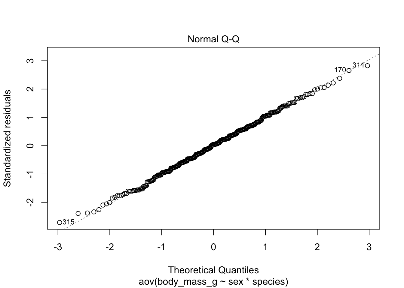
# method 2
library(car)

qqPlot(mod$residuals,
  id = FALSE # remove point identification
)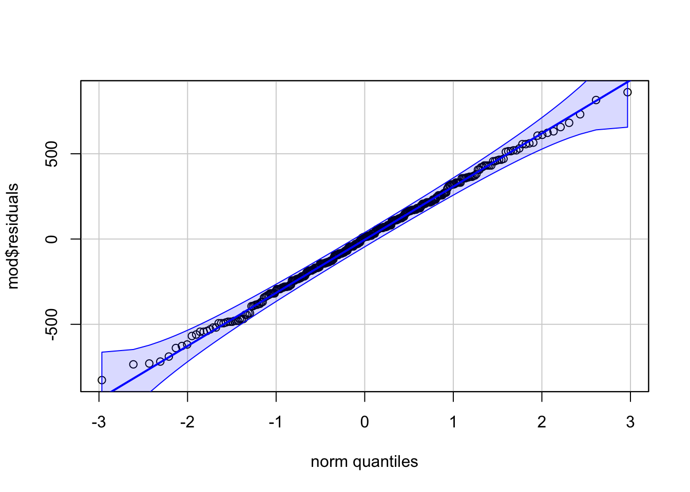
Code for method 1 is slightly shorter, but it misses the confidence interval around the reference line.
If points follow the straight line (called Henry’s line) and fall within the confidence band, we can assume normality. This is the case here.
If you prefer to verify the normality based on a histogram of the residuals, here is the code:
# histogram
hist(mod$residuals)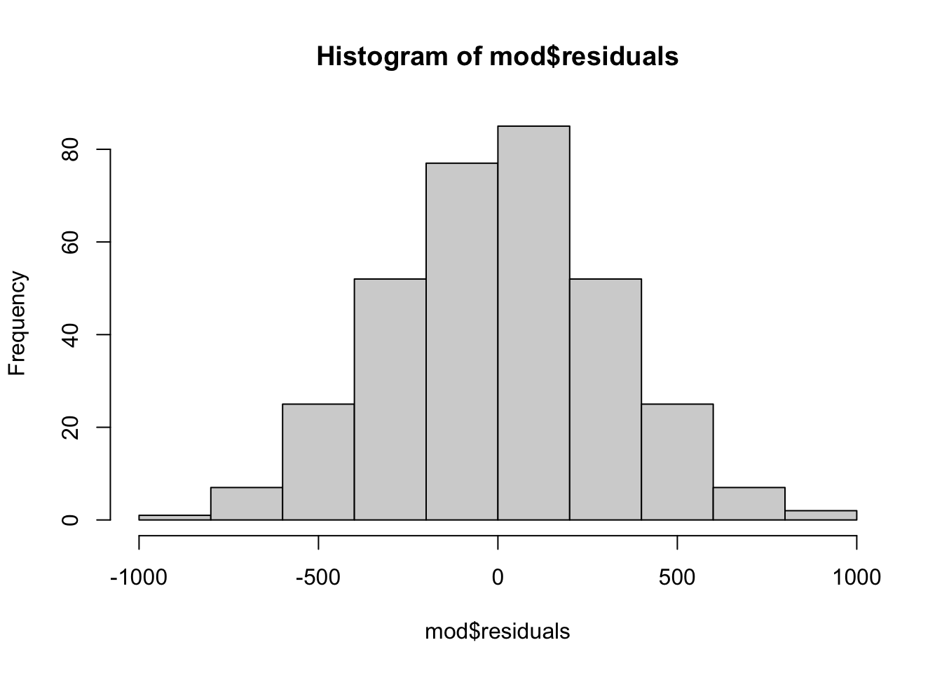
The histogram of the residuals show a gaussian distribution, which is in line with the conclusion from the QQ-plot.
Although the QQ-plot and histogram is largely enough to verify the normality, if you want to test it more formally with a statistical test, the Shapiro-Wilk test can be applied on the residuals as well:
# normality test
shapiro.test(mod$residuals)
##
## Shapiro-Wilk normality test
##
## data: mod$residuals
## W = 0.99776, p-value = 0.9367\(\Rightarrow\) We do not reject the null hypothesis that the residuals follow a normal distribution (\(p\)-value = 0.937).
From the QQ-plot, histogram and Shapiro-Wilk test, we conclude that we do not reject the null hypothesis of normality of the residuals.
The normality assumption is thus verified, we can now check the equality of the variances.
Note that if the normality assumption is not met, many transformations can be applied on the dependent variable to improve it, the most common ones being the logarithmic (log() function in R) and the Box-Cox transformations. If the normality assumption is still not met on the transformed data, the non-parametric version of the two-way ANOVA, the Scheirer–Ray–Hare test, can be used. Alternatively, a permutation test can also be used.
Homogeneity of variances
Equality of variances, also referred as homogeneity of variances or homoscedasticity, can be verified visually with the plot() function:
plot(mod, which = 3)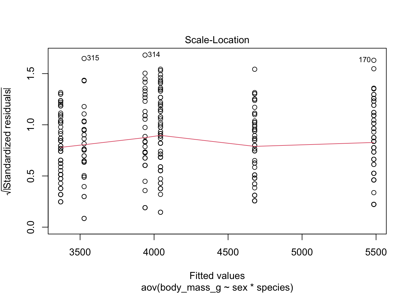
Since the spread of the residuals is constant, the red smooth line is horizontal and flat, so it looks like the constant variance assumption is satisfied here.
The diagnostic plot above is sufficient, but if you prefer it can also be tested more formally with the Levene’s test (also from the {car} package):3
leveneTest(mod)## Levene's Test for Homogeneity of Variance (center = median)
## Df F value Pr(>F)
## group 5 1.3908 0.2272
## 327\(\Rightarrow\) We do not reject the null hypothesis that the variances are equal (\(p\)-value = 0.227).
Both the visual and formal approaches give the same conclusion; we do not reject the hypothesis of homogeneity of the variances.
Note that, as for the normality, the logarithmic and Box-Cox transformations may improve homogeneity of the residuals.
Outliers
The easiest and most common way to detect outliers is visually thanks to boxplots by groups.
For females and males:
library(ggplot2)

# boxplots by sex
ggplot(dat) +
  aes(x = sex, y = body_mass_g) +
  geom_boxplot()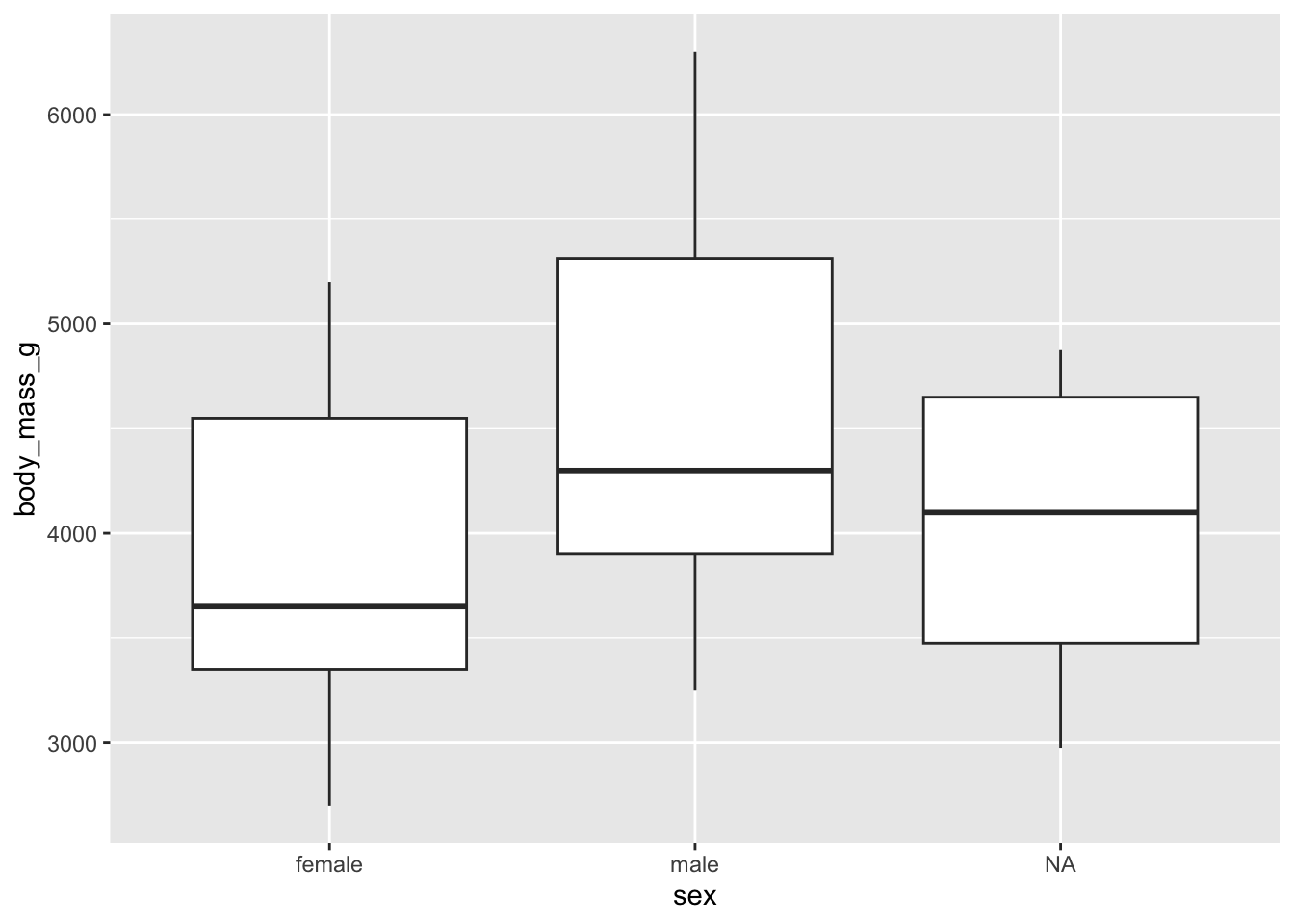
For the three species:
# boxplots by species
ggplot(dat) +
  aes(x = species, y = body_mass_g) +
  geom_boxplot()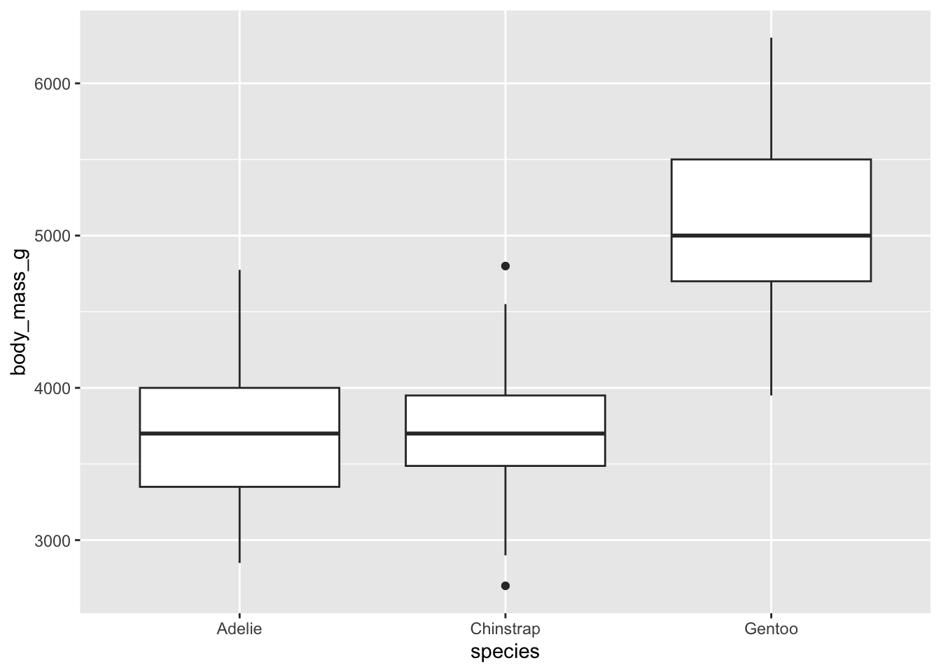
There are, as defined by the interquartile range criterion, two outliers for the species Chinstrap. These points are, nonetheless, not extreme enough to bias results.
Therefore, we consider that the assumption of no significant outliers is met.
Two-way ANOVA
We have shown that all assumptions are met, so we can now proceed to the implementation of the two-way ANOVA in R.
This will allow us to answer the following research questions:
- Controlling for the species, is body mass significantly different between the two sexes?
- Controlling for the sex, is body mass significantly different for at least one species?
- Is the relationship between species and body mass different between female and male penguins?
Preliminary analyses
Before performing any statistical test, it is a good practice to make some descriptive statistics in order to have a first overview of the data, and perhaps, have a glimpse of the results to be expected.
This can be done via descriptive statistics or plots.
Descriptive statistics
If we want to keep it simple, we can compute only the mean for each subgroup:
# mean by group
aggregate(body_mass_g ~ species + sex,
  data = dat,
  FUN = mean
)
## species sex body_mass_g
## 1 Adelie female 3368.836
## 2 Chinstrap female 3527.206
## 3 Gentoo female 4679.741
## 4 Adelie male 4043.493
## 5 Chinstrap male 3938.971
## 6 Gentoo male 5484.836Or eventually, the mean and standard deviation for each subgroup using the {dplyr} package:
# mean and sd by group
library(dplyr)

group_by(dat, sex, species) %>%
  summarise(
    mean = round(mean(body_mass_g, na.rm = TRUE)),
    sd = round(sd(body_mass_g, na.rm = TRUE))
  )
## # A tibble: 8 × 4
## # Groups: sex [3]
## sex species mean sd
## <fct> <fct> <dbl> <dbl>
## 1 female Adelie 3369 269
## 2 female Chinstrap 3527 285
## 3 female Gentoo 4680 282
## 4 male Adelie 4043 347
## 5 male Chinstrap 3939 362
## 6 male Gentoo 5485 313
## 7 <NA> Adelie 3540 477
## 8 <NA> Gentoo 4588 338Plots
If you are a frequent reader of the blog, you know that I like to draw plots to visualize the data at hand before interpreting results of a test.
The most appropriate plot when we have one quantitative and two qualitative variables is a boxplot by group. This can easily be made with the {ggplot2} package:
# boxplot by group
library(ggplot2)

ggplot(dat) +
  aes(x = species, y = body_mass_g, fill = sex) +
  geom_boxplot()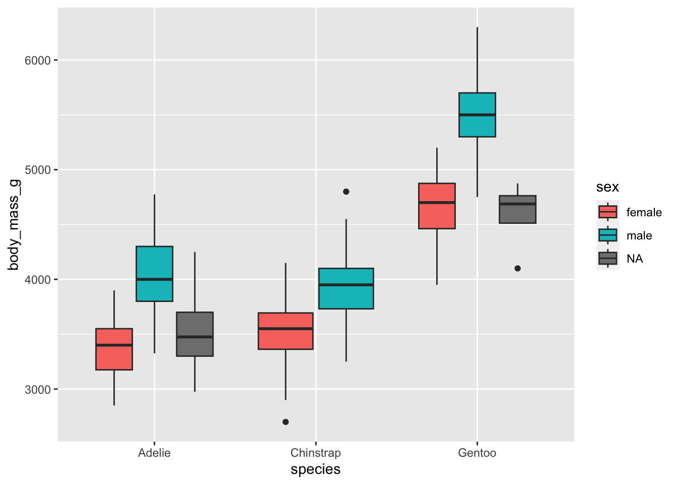
Some observations are missing for the sex, we can remove them to have a more concise plot:
dat %>%
  filter(!is.na(sex)) %>%
  ggplot() +
  aes(x = species, y = body_mass_g, fill = sex) +
  geom_boxplot()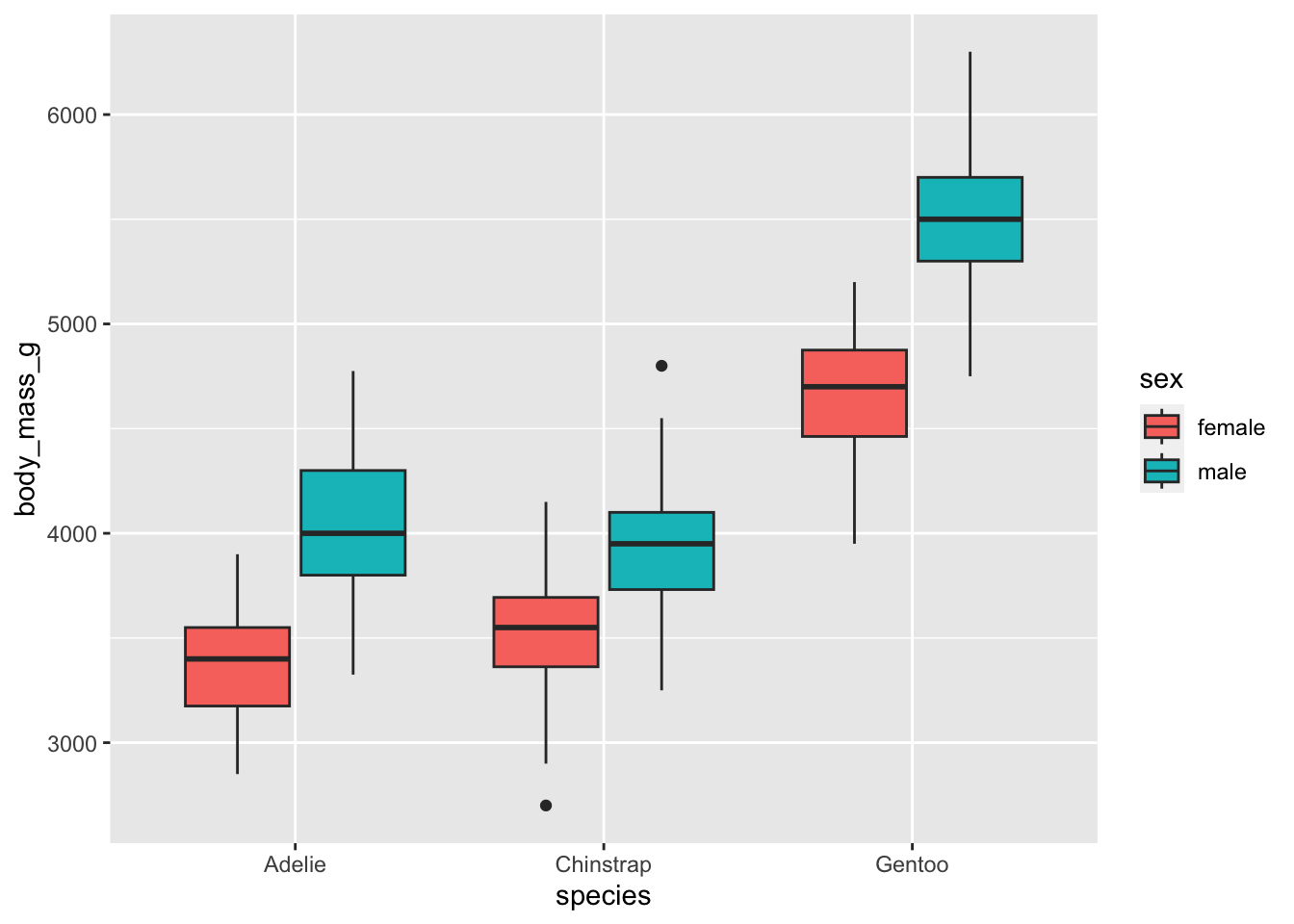
Note that we could also have made the following plot:
dat %>%
  filter(!is.na(sex)) %>%
  ggplot() +
  aes(x = sex, y = body_mass_g, fill = species) +
  geom_boxplot()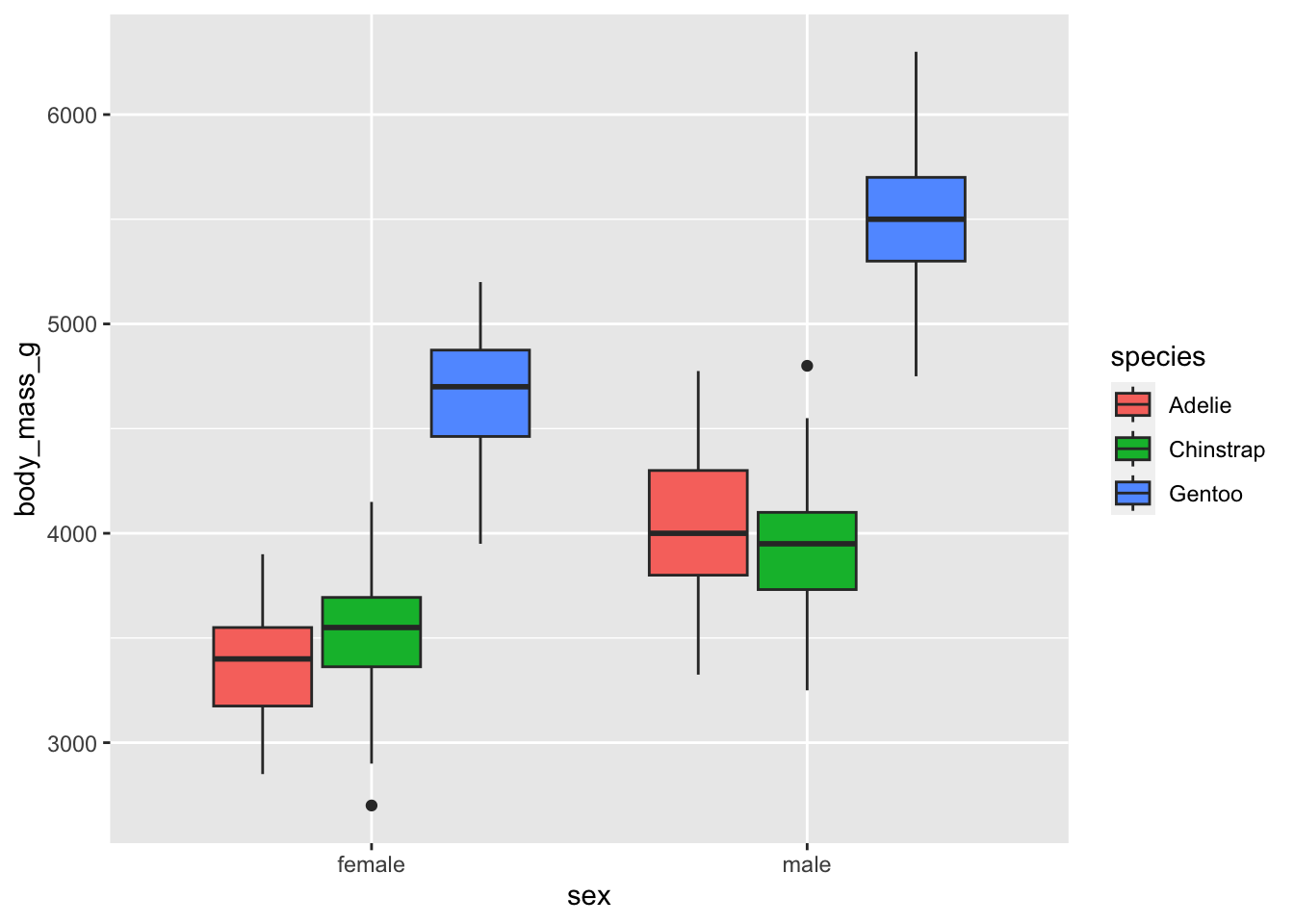
But for a more readable plot, I tend to prefer putting the variable with the smallest number of levels as color (which is in fact the argument fill in the aes() layer) and the variable with the largest number of categories on the x-axis (i.e., the argument x in the aes() layer).
From the means and the boxplots by subgroup, we can already see that, in our sample:
- female penguins tend to have a lower body mass than males, and that is the case for all the considered species, and
- body mass is higher for Gentoo penguins than for the other two species.
Bear in mind that these conclusions are only valid within our sample! To generalize these conclusions to the population, we need to perform the two-way ANOVA and check the significance of the explanatory variables. This is the aim of the next section.
Two-way ANOVA in R
As mentioned earlier, including an interaction effect in a two-way ANOVA is not compulsory. However, in order to avoid flawed conclusions, it is recommended to first check whether the interaction is significant or not, and depending on the results, include it or not.
If the interaction is not significant, it is safe to remove it from the final model. On the contrary, if the interaction is significant, it should be included in the final model which will be used to interpret results.
We thus start with a model which includes the two main effects (i.e., sex and species) and the interaction:
# Two-way ANOVA with interaction
# save model
mod <- aov(body_mass_g ~ sex * species,
  data = dat
)

# print results
summary(mod)
## Df Sum Sq Mean Sq F value Pr(>F)
## sex 1 38878897 38878897 406.145 < 2e-16 ***
## species 2 143401584 71700792 749.016 < 2e-16 ***
## sex:species 2 1676557 838278 8.757 0.000197 ***
## Residuals 327 31302628 95727
## ---
## Signif. codes: 0 '***' 0.001 '**' 0.01 '*' 0.05 '.' 0.1 ' ' 1
## 11 observations deleted due to missingnessSimilar to a one-way ANOVA, the principle of a two-way ANOVA is based on the total dispersion of the data, and its decomposition into four components:
- the share attributable to the first factor
- the share attributable to the second factor
- the share attributable to the interaction of the 2 factors
- the unexplained, or residual portion.
The sum of squares (column Sum Sq) shows these four components. The two-way ANOVA consists of using a statistical test to determine whether each of the dispersion component (attributable to the 2 factors studied and to their interaction) is significantly greater than the residual component. If this is the case, we conclude that the effect considered (factor A, factor B or the interaction) is significant.
We see that the species explain a large part of the variability of body mass. It is the most important factor in explaining this variability.
The \(p\)-values are displayed in the last column of the output above (Pr(>F)). From these \(p\)-values, we conclude that, at the 5% significance level:
- controlling for the species, body mass is significantly different between the two sexes,
- controlling for the sex, body mass is significantly different for at least one species, and
- the interaction between sex and species (displayed at the line
sex:speciesin the output above) is significant.
So from the significant interaction effect, we have just seen that the relationship between body mass and species is different between males and females. Since it is significant, we have to keep it in the model and we should interpret results from that model.
If, on the contrary, the interaction was not significant (that is, if the \(p\)-value \(\ge\) 0.05) we would have removed this interaction effect from the model. For illustrative purposes, below the code for a two-way ANOVA without interaction, referred as an additive model:
# Two-way ANOVA without interaction
aov(body_mass_g ~ sex + species,
  data = dat
)
For the readers who are used to perform linear regressions in R, you will notice that the structure of the code for a two-way ANOVA is in fact similar:
- the formula is
dependent variable ~ independent variables - the
+sign is used to include independent variables without an interaction4 - the
*sign is used to include independent variables with an interaction
The resemblance with a linear regression is not a surprise because a two-way ANOVA, like all ANOVA, is actually a linear model.
Note that the following code works as well, and give the same results:5
# method 2
mod2 <- lm(body_mass_g ~ sex * species,
  data = dat
)

Anova(mod2)
## Anova Table (Type II tests)
##
## Response: body_mass_g
## Sum Sq Df F value Pr(>F)
## sex 37090262 1 387.460 < 2.2e-16 ***
## species 143401584 2 749.016 < 2.2e-16 ***
## sex:species 1676557 2 8.757 0.0001973 ***
## Residuals 31302628 327
## ---
## Signif. codes: 0 '***' 0.001 '**' 0.01 '*' 0.05 '.' 0.1 ' ' 1Note that the aov() function assumes a balanced design, meaning that we have equal sample sizes within levels of our independent grouping variables. Moreover, aov() uses the type I sums of squares, so we can obtain different \(p\)-values when we write y ~ A * B and y ~ B * A.
For unbalanced design, that is, unequal numbers of subjects in each subgroup, the recommended methods are:
- the type II ANOVA when there is no significant interaction, which can be done in R with
Anova(mod, type = "II")orAnova(mod, type = 2), wheremodis the name of your saved model, and - the type III ANOVA when there is a significant interaction, which can be done in R with
Anova(mod, type = "III")orAnova(mod, type = 3).
This is beyond the scope of the post and we assume a balanced design here. For the interested reader, see this detailed discussion about type I, type II and type III ANOVA.
Pairwise comparisons
Through the two main effects being significant, we concluded that:
- controlling for the species, body mass is different between females and males, and
- controlling for the sex, body mass is different for at least one species.
If body mass is different between the two sexes, given that there are exactly two sexes, it must be because body mass is significantly different between females and males.
If one wants to know which sex has the highest body mass, it can be deduced from the means and/or boxplots by subgroup. Here, it is clear that males have a significantly higher body mass than females.
However, it is not so straightforward for the species. Let me explain why it is not as easy as for the sexes.
There are three species (Adelie, Chinstrap and Gentoo), so there are 3 pairs of species:
- Adelie and Chinstrap
- Adelie and Gentoo
- Chinstrap and Gentoo
If body mass is significantly different for at least one species, it could be that:
- body mass is significantly different between Adelie and Chinstrap but not significantly different between Adelie and Gentoo, and not significantly different between Chinstrap and Gentoo, or
- body mass is significantly different between Adelie and Gentoo but not significantly different between Adelie and Chinstrap, and not significantly different between Chinstrap and Gentoo, or
- body mass is significantly different between Chinstrap and Gentoo but not significantly different between Adelie and Chinstrap, and not significantly different between Adelie and Gentoo.
Or, it could also be that:
- body mass is significantly different between Adelie and Chinstrap, and between Adelie and Gentoo, but not significantly different between Chinstrap and Gentoo, or
- body mass is significantly different between Adelie and Chinstrap, and between Chinstrap and Gentoo, but not significantly different between Adelie and Gentoo, or
- body mass is significantly different between Chinstrap and Gentoo, and between Adelie and Gentoo, but not significantly different between Adelie and Chinstrap.
Last, it could also be that body mass is significantly different between all species.
As for a one-way ANOVA, we cannot, at this stage, know precisely which species is different from which one in terms of body mass. To know this, we need to compare each species two by two thanks to post-hoc tests (also known as pairwise comparisons).
There are several post-hoc tests, the most common ones being the Tukey HSD which tests all possible pairs of groups, and the Dunett’s test which compares all groups to a reference group. As mentioned earlier, these tests should not be done on the sex variable because there are only two levels.
In this post, we show only the Tukey HSD test. For the interested reader, the Dunnett’s test is illustrated here.
As for the one-way ANOVA, the Tukey HSD test can be done in R as follows:
# method 1
TukeyHSD(mod,
  which = "species"
)
## Tukey multiple comparisons of means
## 95% family-wise confidence level
##
## Fit: aov(formula = body_mass_g ~ sex * species, data = dat)
##
## $species
## diff lwr upr p adj
## Chinstrap-Adelie 26.92385 -80.0258 133.8735 0.8241288
## Gentoo-Adelie 1377.65816 1287.6926 1467.6237 0.0000000
## Gentoo-Chinstrap 1350.73431 1239.9964 1461.4722 0.0000000or using the {multcomp} package:
# method 2
library(multcomp)

res_tukey <- glht(
  aov(body_mass_g ~ sex + species,
    data = dat
  ),
  linfct = mcp(species = "Tukey")
)

summary(res_tukey)
##
## Simultaneous Tests for General Linear Hypotheses
##
## Multiple Comparisons of Means: Tukey Contrasts
##
##
## Fit: aov(formula = body_mass_g ~ sex + species, data = dat)
##
## Linear Hypotheses:
## Estimate Std. Error t value Pr(>|t|)
## Chinstrap - Adelie == 0 26.92 46.48 0.579 0.83
## Gentoo - Adelie == 0 1377.86 39.10 35.236 <1e-05 ***
## Gentoo - Chinstrap == 0 1350.93 48.13 28.067 <1e-05 ***
## ---
## Signif. codes: 0 '***' 0.001 '**' 0.01 '*' 0.05 '.' 0.1 ' ' 1
## (Adjusted p values reported -- single-step method)or using the pairwise.t.test() function using the \(p\)-value adjustment method of your choice:6
# method 3
pairwise.t.test(dat$body_mass_g, dat$species,
  p.adjust.method = "BH"
)
##
## Pairwise comparisons using t tests with pooled SD
##
## data: dat$body_mass_g and dat$species
##
## Adelie Chinstrap
## Chinstrap 0.63 -
## Gentoo <2e-16 <2e-16
##
## P value adjustment method: BHNote that when using the second method, it is the model without the interaction that needs to be specified into the glht() function, even if the interaction is significant. Moreover, do not forget to replace mod and species in my code with the name of your model and the name of your independent variable.
Both methods give the same results, that is:
- body mass is not significantly different between Chinstrap and Adelie (adjusted \(p\)-value = 0.83),
- body mass is significantly different between Gentoo and Adelie (adjusted \(p\)-value < 0.001), and
- body mass is significantly different between Gentoo and Chinstrap (adjusted \(p\)-value < 0.001).
Remember that it is the adjusted \(p\)-values that are reported, to prevent the issue of multiple testing which occurs when comparing several pairs of groups.
If you would like to compare all combinations of groups, it can be done with the TukeyHSD() function and specifying the interaction in the which argument:
# all combinations of sex and species
TukeyHSD(mod,
  which = "sex:species"
)
## Tukey multiple comparisons of means
## 95% family-wise confidence level
##
## Fit: aov(formula = body_mass_g ~ sex * species, data = dat)
##
## $`sex:species`
## diff lwr upr p adj
## male:Adelie-female:Adelie 674.6575 527.8486 821.4664 0.0000000
## female:Chinstrap-female:Adelie 158.3703 -25.7874 342.5279 0.1376213
## male:Chinstrap-female:Adelie 570.1350 385.9773 754.2926 0.0000000
## female:Gentoo-female:Adelie 1310.9058 1154.8934 1466.9181 0.0000000
## male:Gentoo-female:Adelie 2116.0004 1962.1408 2269.8601 0.0000000
## female:Chinstrap-male:Adelie -516.2873 -700.4449 -332.1296 0.0000000
## male:Chinstrap-male:Adelie -104.5226 -288.6802 79.6351 0.5812048
## female:Gentoo-male:Adelie 636.2482 480.2359 792.2606 0.0000000
## male:Gentoo-male:Adelie 1441.3429 1287.4832 1595.2026 0.0000000
## male:Chinstrap-female:Chinstrap 411.7647 196.6479 626.8815 0.0000012
## female:Gentoo-female:Chinstrap 1152.5355 960.9603 1344.1107 0.0000000
## male:Gentoo-female:Chinstrap 1957.6302 1767.8040 2147.4564 0.0000000
## female:Gentoo-male:Chinstrap 740.7708 549.1956 932.3460 0.0000000
## male:Gentoo-male:Chinstrap 1545.8655 1356.0392 1735.6917 0.0000000
## male:Gentoo-female:Gentoo 805.0947 642.4300 967.7594 0.0000000Or with the HSD.test() function from the {agricolae} package, which denotes subgroups that are not significantly different from each other with the same letter:
library(agricolae)

HSD.test(mod,
  trt = c("sex", "species"),
  console = TRUE # print results
)
##
## Study: mod ~ c("sex", "species")
##
## HSD Test for body_mass_g
##
## Mean Square Error: 95726.69
##
## sex:species, means
##
## body_mass_g std r Min Max
## female:Adelie 3368.836 269.3801 73 2850 3900
## female:Chinstrap 3527.206 285.3339 34 2700 4150
## female:Gentoo 4679.741 281.5783 58 3950 5200
## male:Adelie 4043.493 346.8116 73 3325 4775
## male:Chinstrap 3938.971 362.1376 34 3250 4800
## male:Gentoo 5484.836 313.1586 61 4750 6300
##
## Alpha: 0.05 ; DF Error: 327
## Critical Value of Studentized Range: 4.054126
##
## Groups according to probability of means differences and alpha level( 0.05 )
##
## Treatments with the same letter are not significantly different.
##
## body_mass_g groups
## male:Gentoo 5484.836 a
## female:Gentoo 4679.741 b
## male:Adelie 4043.493 c
## male:Chinstrap 3938.971 c
## female:Chinstrap 3527.206 d
## female:Adelie 3368.836 dIf you have many groups to compare, plotting them might be easier to interpret:
# set axis margins so labels do not get cut off
par(mar = c(4.1, 13.5, 4.1, 2.1))

# create confidence interval for each comparison
plot(TukeyHSD(mod, which = "sex:species"),
  las = 2 # rotate x-axis ticks
)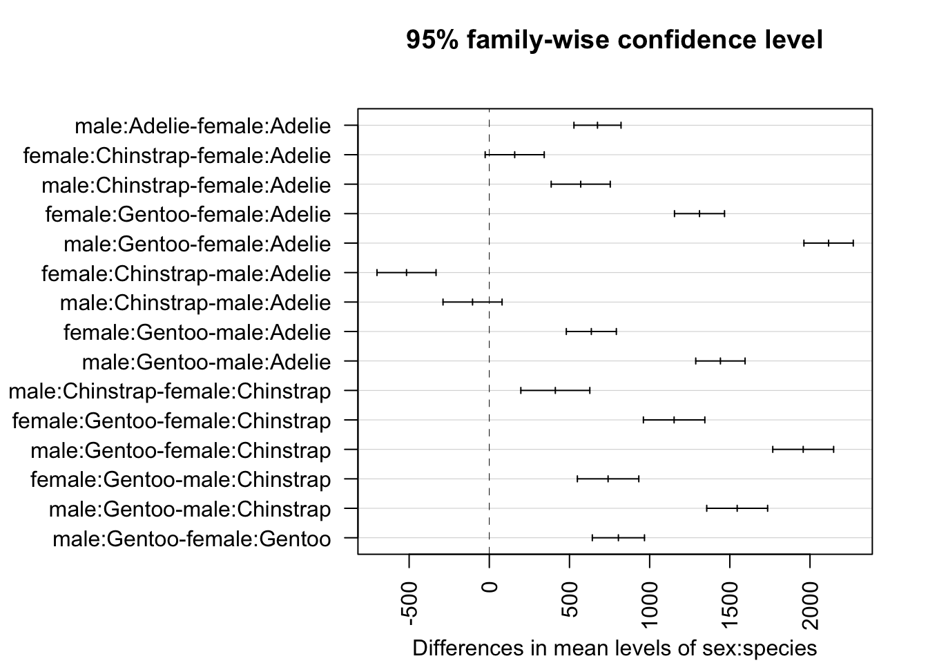
From the outputs and plot above, we conclude that all combinations of sex and species are significantly different, except between female Chinstrap and female Adelie (\(p\)-value = 0.138) and male Chinstrap and male Adelie (\(p\)-value = 0.581).
These results, which are by the way in line with the boxplots shown above and which will be confirmed with the visualizations below, concludes the two-way ANOVA in R.
Visualizations
If you would like to visualize results in a different way to what has already been presented in the preliminary analyses, below are some ideas of useful plots.
First, with the mean and standard error of the mean by subgroup using the allEffects() function from the {effects} package:
# method 1
library(effects)

plot(allEffects(mod))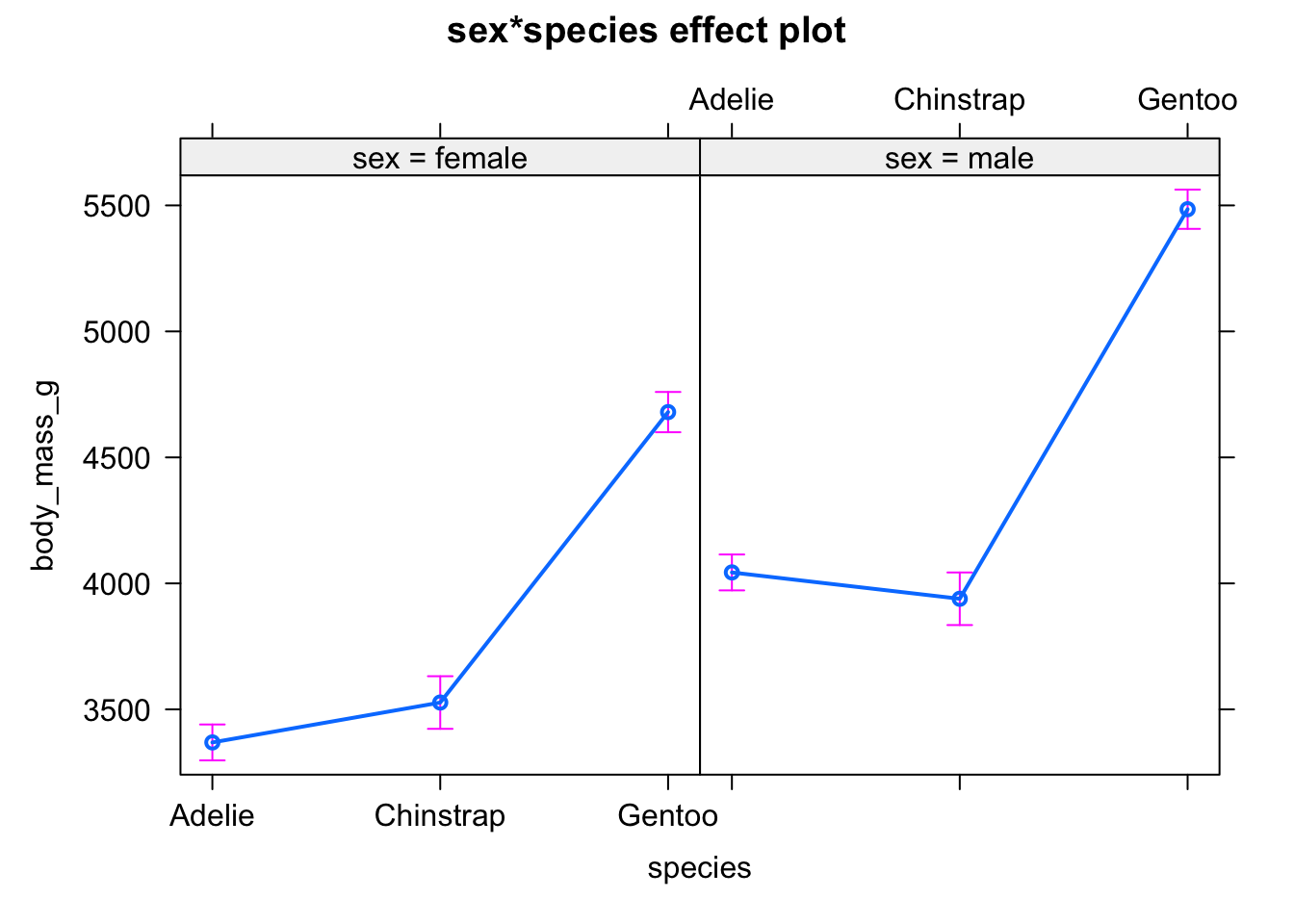
Or using the {ggpubr} package:
# method 2
library(ggpubr)

ggline(subset(dat, !is.na(sex)), # remove NA level for sex
  x = "species",
  y = "body_mass_g",
  color = "sex",
  add = c("mean_se") # add mean and standard error
) +
  labs(y = "Mean of body mass (g)")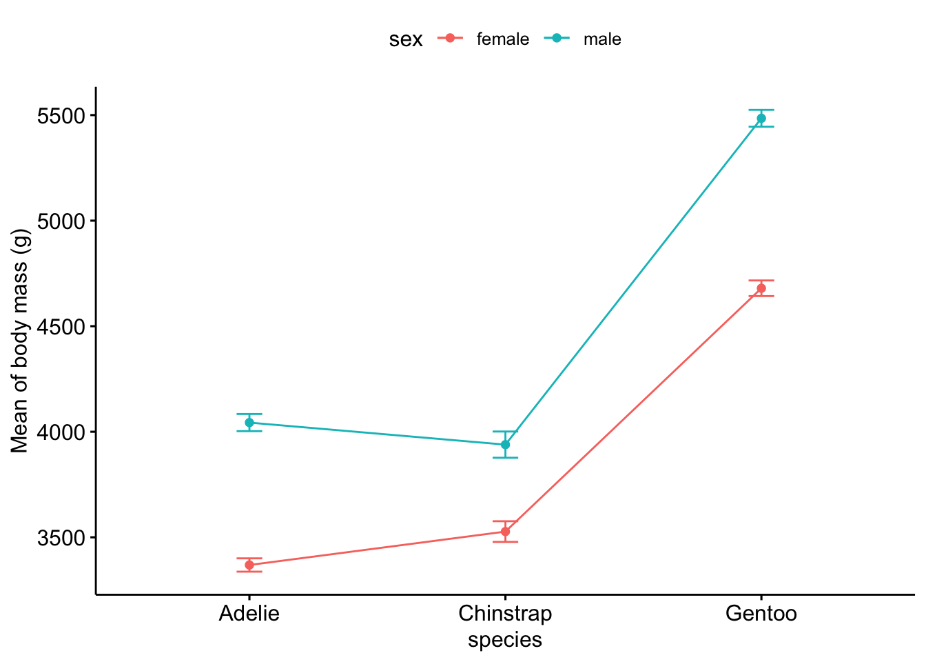
Alternatively, using {Rmisc} and {ggplot2}:
library(Rmisc)

# compute mean and standard error of the mean by subgroup
summary_stat <- summarySE(dat,
  measurevar = "body_mass_g",
  groupvars = c("species", "sex")
)

# plot mean and standard error of the mean
ggplot(
  subset(summary_stat, !is.na(sex)), # remove NA level for sex
  aes(x = species, y = body_mass_g, colour = sex)
) +
  geom_errorbar(aes(ymin = body_mass_g - se, ymax = body_mass_g + se), # add error bars
    width = 0.1 # width of error bars
  ) +
  geom_point() +
  labs(y = "Mean of body mass (g)")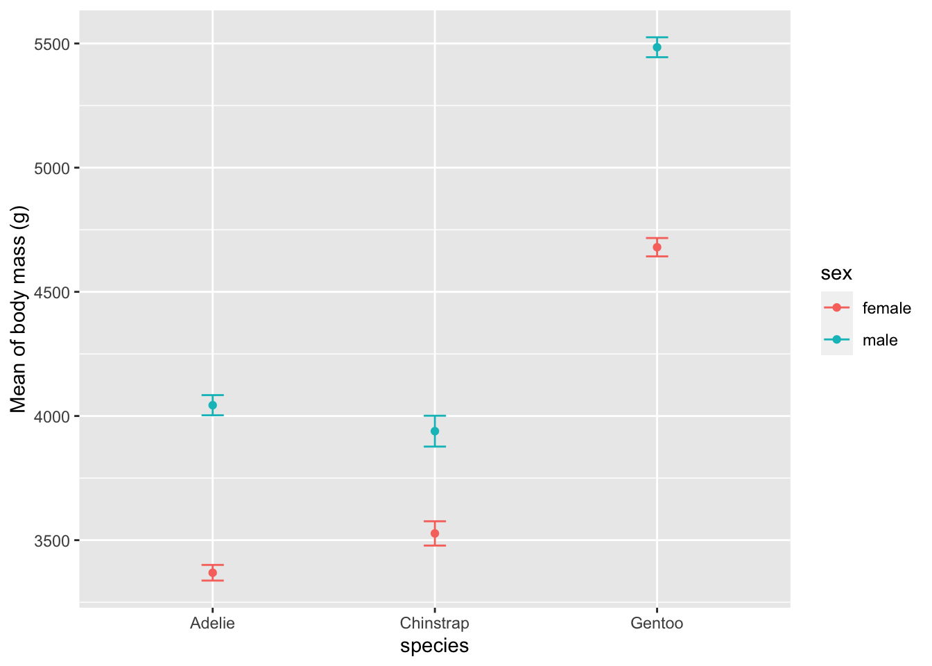
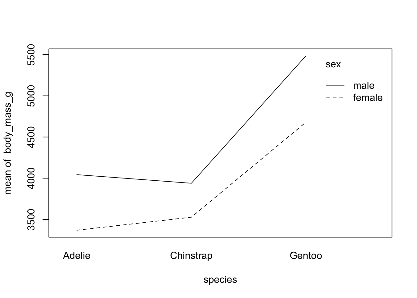
Second, if you prefer to draw only the mean by subgroup:
with(
  dat,
  interaction.plot(species, sex, body_mass_g)
)
Last but not least, for those of you who are familiar with GraphPad, you are most likely familiar with plotting means and error bars as follows:
# plot mean and standard error of the mean as barplots
ggplot(
  subset(summary_stat, !is.na(sex)), # remove NA level for sex
  aes(x = species, y = body_mass_g, fill = sex)
) +
  geom_bar(position = position_dodge(), stat = "identity") +
  geom_errorbar(aes(ymin = body_mass_g - se, ymax = body_mass_g + se), # add error bars
    width = 0.25, # width of error bars
    position = position_dodge(.9)
  ) +
  labs(y = "Mean of body mass (g)")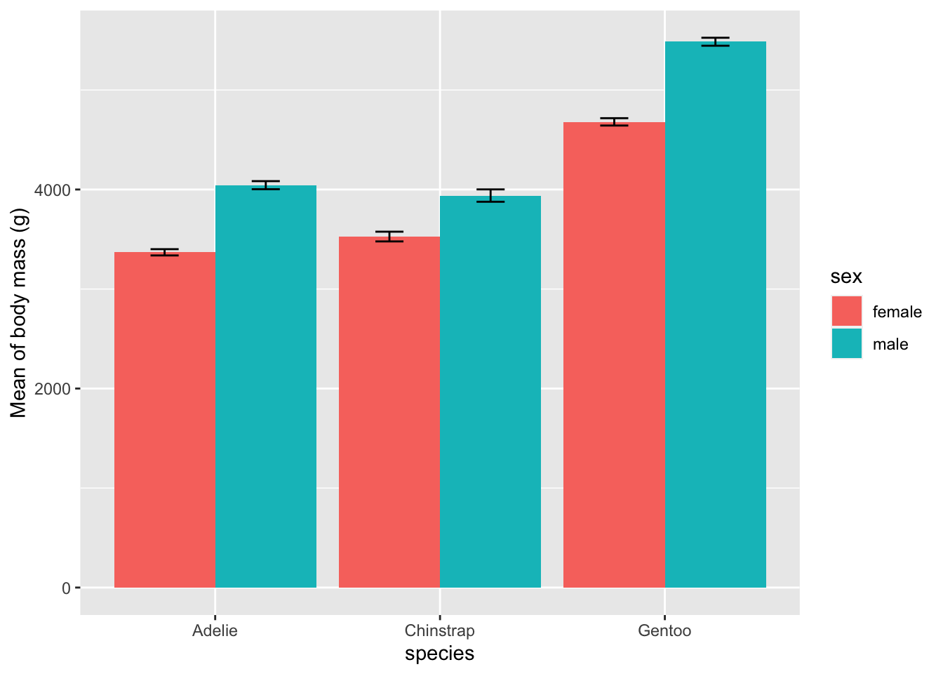
Conclusion
In this post, we started with a few reminders of the different tests that exist to compare a quantitative variable across groups. We then focused on the two-way ANOVA, starting from its goal and hypotheses to its implementation in R, together with the interpretations and some visualizations. We also briefly mentioned its underlying assumptions and one post-hoc test to compare all subgroups.
All this was illustrated with the penguins dataset available from the {palmerpenguins} package.
Thanks for reading.
I hope this article will help you in conducting a two-way ANOVA with your data.
As always, if you have a question or a suggestion related to the topic covered in this article, please add it as a comment so other readers can benefit from the discussion.
In theory, a one-way ANOVA can also be used to compare 2 groups, and not only 3 or more. Nonetheless, in practice, it is often the case that a Student’s t-test is performed to compare 2 groups, and a one-way ANOVA to compare 3 or more groups. Conclusions obtained via a Student’s t-test for independent samples and a one-way ANOVA with 2 groups will be similar.↩︎
If you really want to test the independence, you can do so visually with a plot of the residuals vs. fitted values. This plot can be done in R with
plot(mod, which = 1), wheremodcorresponds to the name of your model. Or you can do so with the Durbin-Watson test. In R, it can be done with thedurbinWatsonTest()function from the{car}package.↩︎Note that the Bartlett’s and Fligner-Killeen tests are also appropriate to test the assumption of equal variances.↩︎
An additive model makes the assumption that the 2 explanatory variables are independent; they do not interact with each other.↩︎
To not be confused with the
anova()function because it provides sequential results that depend on the order in which the variables appear in the model.↩︎Here, we use the Benjamini & Hochberg (1995) correction, but you can choose between several methods. See
?p.adjustfor more details.↩︎
Liked this post?
- Get updates every time a new article is published (no spam and unsubscribe anytime)
- Support the blog
- Share on:


