Introduction

In a previous article, we showed how to do a two-sample Wilcoxon test in R. Remember that there are actually two versions of this test:

1. The Mann-Whitney-Wilcoxon test (also referred as Wilcoxon rank sum test or Mann-Whitney U test), used to compare two independent samples. This test is the non-parametric version of the Student’s t-test for independent samples.
2. The Wilcoxon signed-rank test (also referred as Wilcoxon test for paired samples), used to compare two paired samples. This test is the non-parametric version of the Student’s t-test for paired samples.

In another article, we also showed how to do a one-sample t-test by hand and in R. This test is used to determine whether the mean of a measurement variable is different from a specified value (a value that you specify based on your beliefs or a theoretical expectation for example). Since it is a parametric test, the data should follow a normal distribution (or sample size should be large enough (i.e., above 30), thanks to the central limit theorem) for the results to be valid.

Unlike the one-sample t-test, the one-sample Wilcoxon test (also referred as the one-sample Wilcoxon signed-rank test) is a non-parametric test, meaning that it does not rely on data belonging to any particular parametric family of probability distributions. Non-parametric tests usually have the same goal as their parametric counterparts (in this case, compare data to a given value). Nonetheless, they do not require the assumption of normality and they can deal with outliers and Likert scales.

In this article, we show when to perform the one-sample Wilcoxon test, how to do it in R and how to interpret its results. We will also briefly show some appropriate visualizations.

When?

The one-sample Wilcoxon test is used to compare our observations to a given default value—a value that you specify based on your beliefs or a theoretical expectation for example. In other words, it is used to determine if a group is significantly different from a known or hypothesized population value on the variable of interest.

Since the test statistic is computed based on the ranks of the difference between the observed values and the default value (making it a non-parametric test), the one-sample Wilcoxon test is more appropriate than a one-sample t-test when the observations do not follow a normal distribution.

The goal of this test is to verify whether the observations are significantly different from our default value. In terms of null and alternative hypotheses, we have (for a two-tailed test):

• \(H_0:\) location of the data is equal to the chosen value
• \(H_1:\) location of the data is different from the chosen value

In other words, a significant result (i.e., a rejection of the null hypothesis) suggests that the location of the data is different from the chosen value.

Note that some authors suggest that this test is a test of the median, that is (for a two-tailed test):

• \(H_0:\) the median is equal to the chosen value
• \(H_1:\) the median is different from the chosen value

However, this is the case only if the data are symmetric. Without further assumptions about the distribution of the data, the one-sample Wilcoxon test is not a test of the median but a test about the location of the data.¹

Note that although the normality assumption is not required, the independence assumption must still be verified. This means that observations must be independent of one another (usually, random sampling is sufficient to have independence).

Data

For our illustration, suppose we want to test whether the scores at an exam differ from 10, that is:

• \(H_0:\) scores at the exam \(= 10\)
• \(H_1:\) scores at the exam \(\ne 10\)

To verify this, we have a sample of 15 students and their score at the exam:

dat

##    Student_ID Score
## 1           1    17
## 2           2     5
## 3           3     1
## 4           4    10
## 5           5     4
## 6           6    18
## 7           7    17
## 8           8    15
## 9           9     7
## 10         10     4
## 11         11     5
## 12         12    14
## 13         13    20
## 14         14    18
## 15         15    15

Scores between students are assumed to be independent (a student’s score is not impacted or influenced by the score of another student). Therefore, the independence assumption is met.

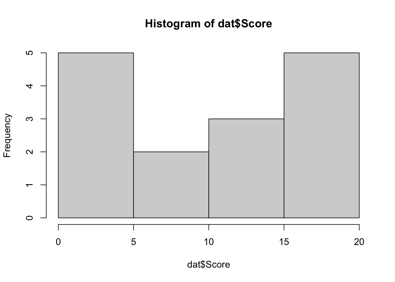
Moreover, sample size is small (n < 30) and based on the histogram the data do not follow a normal distribution:

# histogram
hist(dat$Score)

Note that we refrain from verifying the normality via a normality test (such as the Shapiro-Wilk test for instance) because for small sample sizes, normality tests have little power to reject the null hypothesis and therefore small samples most often pass normality tests (Öztuna, Elhan, and Tüccar 2006; Ghasemi and Zahediasl 2012).

Note also that although we use a quantitative variable for the illustration, the one-sample Wilcoxon test is also appropriate for interval data and Likert scales.

How?

The one-sample Wilcoxon test can be done in R with the wilcox.test() function.

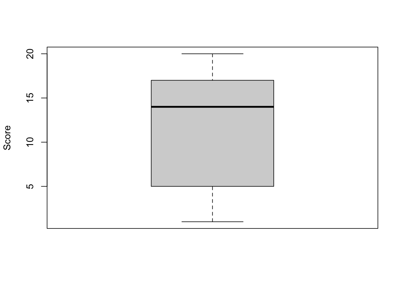
But first, it is a good practice to visualize our data in a boxplot and compute some descriptive statistics to compare our observations with our default value:

# boxplot
boxplot(dat$Score,
  ylab = "Score"
)

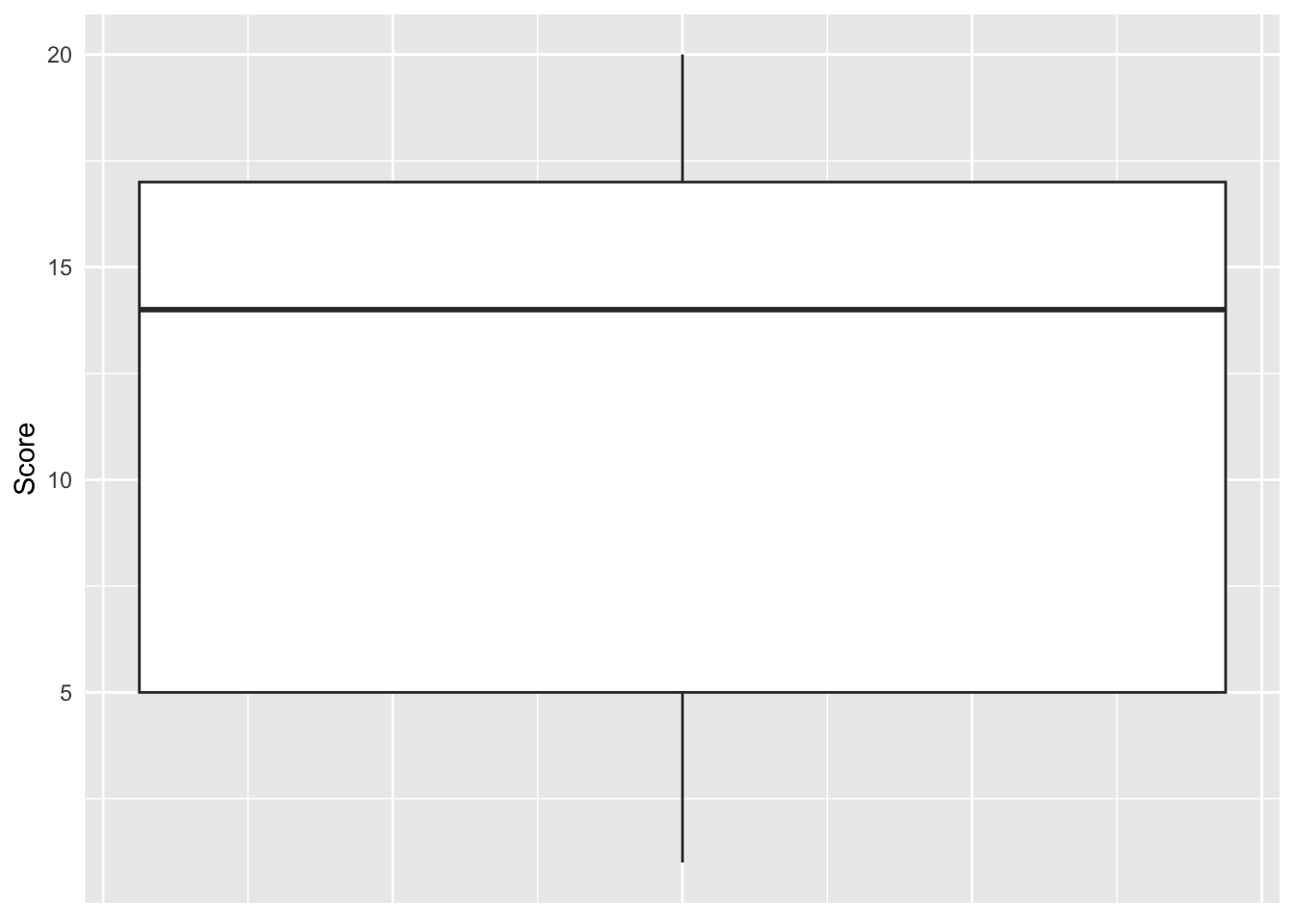
If like me you prefer to use the {ggplot2} package for your plots:

# boxplot
library(ggplot2)

ggplot(dat, aes(y = Score)) +
  geom_boxplot() +
  labs(y = "Score") +
  theme( # remove axis text and ticks
    axis.text.x = element_blank(),
    axis.ticks = element_blank()
  )

Some basic descriptive statistics (rounded to two decimals):

round(summary(dat$Score),
  digits = 2
)

##    Min. 1st Qu.  Median    Mean 3rd Qu.    Max. 
##    1.00    5.00   14.00   11.33   17.00   20.00

From the boxplot and the descriptive statistics above, we see that the mean and median of the scores in our sample are respectively 11.33 and 14.

The one-sample Wilcoxon test will tell us whether the scores are significantly different from 10 or not (and thus whether they are different from 10 in the population or not):

wilcox.test(dat$Score,
  mu = 10 # default value
)

## 
##  Wilcoxon signed rank test with continuity correction
## 
## data:  dat$Score
## V = 67, p-value = 0.3779
## alternative hypothesis: true location is not equal to 10

The output presents several information such as the:

• title of the test
• data
• test statistic
• \(p\)-value
• alternative hypothesis

We focus on the \(p\)-value to interpret and conclude the test.

Interpretation:

Based on the results of the test, (at the significance level of 0.05) we do not reject the null hypothesis, so we do not reject the hypothesis that the scores at this exam are equal to 10, and we cannot conclude that the scores are significantly different from 10 (\(p\)-value = 0.378).

By default, it is a two-tailed test that is done. As for the t.test() function, we can specify that a one-sided test is required by using either the alternative = "greater" or alternative = "less argument in the wilcox.test() function.

For example, if we want to test that the scores are higher than 10:

wilcox.test(dat$Score,
  mu = 10, # default value
  alternative = "greater" # H1: scores > 10
)

## 
##  Wilcoxon signed rank test with continuity correction
## 
## data:  dat$Score
## V = 67, p-value = 0.189
## alternative hypothesis: true location is greater than 10

Interpretation:

In this case, we still do not reject the hypothesis that scores are equal to 10 and we cannot conclude that scores are significantly higher than 10 (\(p\)-value = 0.189).

For more information about the arguments available in the function, see ?wilcox.test.

Note that you may encounter the following warnings when using wilcox.test():

Warning messages:
1: In wilcox.test.default(dat$Score, mu = 10) :
  cannot compute exact p-value with ties
2: In wilcox.test.default(dat$Score, mu = 10) :
  cannot compute exact p-value with zeroes

It is a warning rather than an indication that your results are incorrect. R is informing you that it is reporting a \(p\)-value based on a normal approximation rather than an exact \(p\)-value based on the data because there are ties (some values are the same). Use the exact = FALSE option if you want to remove the warning.

Combine statistical test and plot

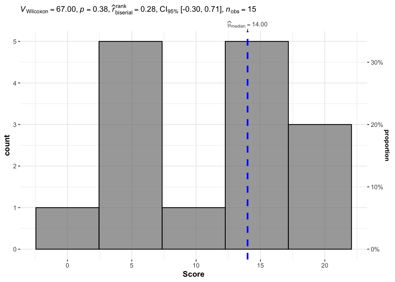
If you are a frequent user of the blog, you know that I like to present results of a test directly on a plot. This allows me to visualize the data and conclude the test in a concise manner.

This is possible thanks to the gghistostats() function within the {ggstatsplot} package:

# load package
library(ggstatsplot)

# combine plot and test
gghistostats(
  data = dat, # dataframe
  x = Score, # variable
  type = "nonparametric", # nonparemetric = Wilcoxon, parametric = t-test
  test.value = 10 # default value
)

The histogram² shows the distribution of the scores and results of the test is shown in the title of the plot.

As you can see, results of the test are the same, that is, there is not enough evidence in the data to conclude that scores are significantly different from 10 (\(p\)-value = 0.378).

Conclusion

Thanks for reading.

I hope this article helped you to understand the one-sample Wilcoxon test and how to do it in R.

As always, if you have any question related to the topic covered in this paper, please add it as a comment so other readers can benefit from the discussion.