What is survival analysis? Examples by hand and in R

Note that this article is inspired from:
- the lecture notes of Prof. Van Keilegom and my personal notes as teaching assistant for her course entitled “Analysis of Survival and Duration Data” given at UCLouvain
- the lecture notes of Prof. Legrand for her course entitled “Statistics in clinical trials” given at UCLouvain
Introduction
For the last post of the year, I would like to present a rather unknown (yet important) statistical method–survival analysis.
Although survival analysis is a branch of statistics, it is usually not covered in introductory statistics courses and it is rather unknown to the general public. It is mostly taught in biostatistics courses or advanced statistics study programs.
In this article, I will explain what is survival analysis, in which context and how it is used. I will explain the main tools and methods used by biostatisticians to analyze survival data and how to estimate and interpret survival curves.
I will show in detail how to apply these techniques in R with concrete examples. In practice, survival analysis is almost always done via a statistical program and never done by hand. However, as for any statistical concept, I believe that doing it by hand allows to really understand the concepts and what these programs actually do. For this reason, I will also show a brief example on how to perform a basic survival analysis by hand.
What is survival analysis?
Survival analysis (also called time-to-event analysis or duration analysis) is a branch of statistics aimed at analyzing the duration of time from a well-defined time origin until one or more events happen, called survival times or duration times.
In other words, in survival analysis, we are interested in a certain event and want to analyze the time until the event happens.
While the event of interest is often death (in this case we study the time to death for patients having a specific disease) or recurrence (in this case we study the time to relapse of a certain disease), it is not limited to the medical field or epidemiology.
In fact, it can be used in many domains. For example, we may also analyze the time until:
- getting cured from a certain disease
- finding a new job after a period of unemployment
- being arrested again after having been released from jail
- the first pregnancy
- the failure of a mechanical system or a machine
- a bank or a company goes bankrupt
- a customer buys a new product or stops its current subscription
- a letter is delivered
- a taxi picks you up after having called the taxi company
- an employee leaves the company
- etc.
As you can see, the event of interest does not necessarily have to be the death or the occurrence of a disease, but in all situations we are interested in analyzing the time until a specific event occurs.
Why do we need special methods for survival analysis?
Survival data, also referred as time-to-event data, requires a special set of statistical methods for three main reasons:
- Duration times are always positive: the time until an event of interest occurs cannot be less than 0. Moreover, the distribution of survival times is right-skewed.
- Different measures are of interest depending on the research question, context, etc. For instance, we could be interested in:
- The probability that a cancer patient survives longer than 5 years after diagnosis?
- The typical waiting time for a cab to arrive after having called the taxi company?
- How many, out of 100 unemployed people, are expected to have a job again after 2 months of unemployment?
- Censoring is almost always an issue:
- When the event occurred before the end of the study, the survival time is known.
- However, sometimes, the event is not yet observed at the end of the study. Suppose that we study the time until death of patients with breast cancer. Luckily, some patients will not die before the end of the study.
- It can also happen that the patient withdraws from the study or moves to another country before the end of the study (known as lost to follow up or drop out).
- In all situations, his or her survival time cannot be observed because the event is not observed for the duration of the study.
- Censoring can be seen, in some sense, as a type of missing data.
- For these reasons, many “standard” statistical tools such as descriptive statistics, hypothesis tests and regression models are not appropriate for this kind of data. Specific statistical methods are required to take into account the fact that the exact survival duration for some patients is missing. It is known that they survived a certain amount of time (until the end of the study or until the time of withdrawal), but their exact survival time is unknown.
For your information, there are three types of censoring:
- right-censoring (the most frequent),
- left-censoring (the least frequent) and
- interval-censoring.
When the event is not yet observed at the end of the study (i.e., the survival time is greater than the observed duration), this is referred as right-censoring. Left-censoring occurs if a participant is entered into the study when the event of interest occurred prior to study entry but we do not know exactly when. Interval-censoring implies that the event occurred within a time interval (between two known dates, two visits, etc.); the exact moment of occurrence is not known. The goal is of course to analyze all available data, including information about censored patients.
The goal of survival analysis is thus to model and describe time-to-event data in an appropriate way, taking the particularities of this type of data into account.
Common functions in survival analysis
We are not going to go to much into the details, but it is important to lay the foundation with the most common functions in survival analysis.
Let \(T\) be a non-negative continuous random variable, representing the time until the event of interest. We consider the following functions:
- Survival function
- Cumulative hazard function
- Hazard function
Survival function
The most common one is the survival function.
Let \(T\) be a non-negative continuous random variable, representing the time until the event of interest. The survival function \(S(t)\) is the probability that a randomly chosen individual is still at risk at time \(t\), where \(0 \le t \le +\infty\). For each \(t\), it is given by
\[ \begin{align*} S(t) &= P(T > t)\\ &= 1 - P(T \le t)\\ &= 1 - F(t)\\ &= 1 - \int^t_0 f(u)\text{d}u, \end{align*} \]
where \(f(\cdot)\) and \(F(\cdot)\) are the density and the cumulative distribution functions of \(T\), respectively.
\(S(t)\) represents, for each time \(t\), the probability that the time until the event is greater than this time \(t\). In other words, it models the probability that the event of interest happens after \(t\).
In the context of our examples mentioned above, it gives the probability that:
- a randomly selected patient will survive beyond time \(t\) or the proportion of patients still alive after time \(t\),
- a cab takes more than \(t\) minutes to arrive, or
- an unemployed person take more than \(t\) months to find a new job.
The survival function \(S(t)\) is:
- a decreasing function,
- taking values in \([0, 1]\) (since it is a probability), and
- equal to 1 at \(t = 0\) (i.e., \(S(0) = 1\)) and 0 at \(t = \infty\) (i.e., \(S(\infty) = 0\)).
Visually we have:
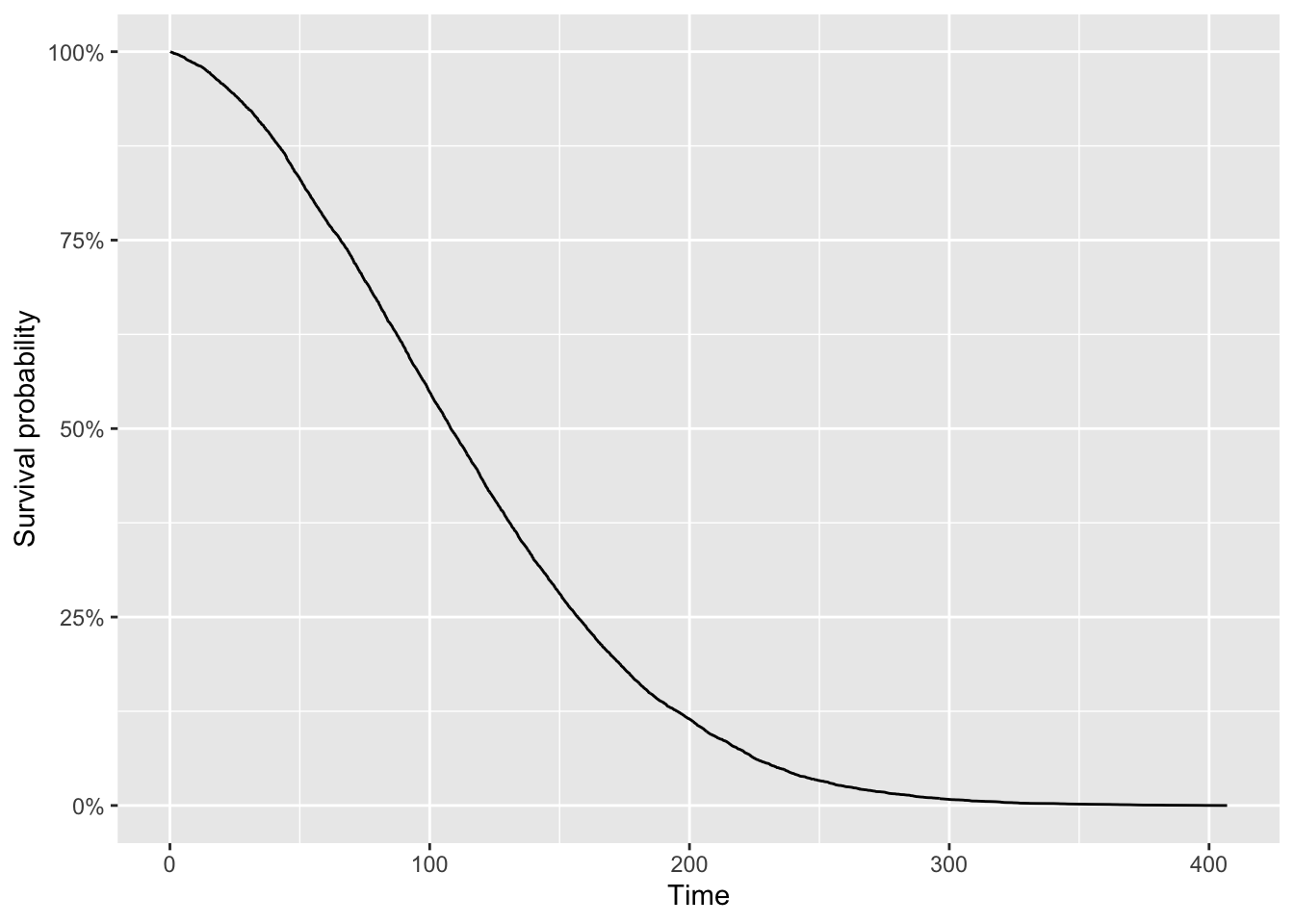
The curve shows the proportion of individuals (or experimental units) who, as time goes on, have not experienced the event of interest. As time progresses, events occur, so the proportion who have not experienced the event decreases.
Cumulative hazard function
The cumulative hazard function, which is the total hazard experienced up to time \(t\), is defined as:
\[H(t) = -log\left(S(t)\right)\]
and has the following properties:
- increasing function,
- taking value in \([0, +\infty]\), and
- \(S(t) = exp(-H(t))\).
Hazard function
The hazard function \(h(t)\), or hazard rate, defines the instantaneous event rate at time \(t\) for an individual still at risk at that time. It can be obtained by
\[ \begin{align*} h(t) &= \lim_{\Delta t \rightarrow 0} \frac{P(t \le T < t + \Delta t | T \ge t)}{\Delta t}\\ &= \frac{d}{dt} H(t)\\ &= \frac{f(t)}{S(t)}. \end{align*} \]
and has the following properties:
- positive function (not necessarily increasing or decreasing)
- the hazard function \(h(t)\) can have many different shapes and is therefore a useful tool to summarize survival data
In the context of cancer research when death is the event of interest, \(h(t)\) measures the instantaneous risk of dying right after time \(t\) given the individual is alive at time \(t\).
To link the hazard rate with the survival function; the survival curve represents the hazard rates. A steeper slope indicates a higher hazard rate because events happen more frequently, reducing the proportion of individuals who have not experienced the event at a faster rate. On the contrary, a gradual and flatter slope indicates a lower hazard rate because events occur less frequently, reducing the proportion of individuals who have not experiences the event at a slower rate. More formally:
\[S(t) = \exp\left(-\int^t_0 h(u) \text{d}u\right).\]
Note that, in contrast to the survival function which focuses on not having an event, the hazard function focuses on the event occurring.
Estimation
To estimate the survival function, we need to use an estimator which is able to deal with censoring. The most common one is the nonparametric Kaplan and Meier (1958) estimator (also sometimes referred as the product-limit estimator, or more simply, the K-M estimator).
The advantages of the Kaplan-Meier estimator are that:
- it is simple and straightforward to use and interpret
- it is a nonparametric estimator, so it constructs a survival curve from the data and no assumptions is made about the shape of the underlying distribution
- it gives a graphical representation of the survival function(s), useful for illustrative purposes
The principle behind this estimator is that surviving beyond time \(t_i\) implies surviving beyond time \(t_{i-1}\) and surviving at time \(t_i\). Note that an important assumption for the estimation to hold is that censoring is independent of the occurrence of events. We say that censoring is non-informative, that is, censored subjects have the same survival prospects as subjects who are not censored and who continue to be followed.
By hand
To understand how it works, let’s first estimate it by hand on the following dataset:1
| subject | time | event |
|---|---|---|
| 1 | 3 | 0 |
| 2 | 5 | 1 |
| 3 | 7 | 1 |
| 4 | 2 | 1 |
| 5 | 18 | 0 |
| 6 | 16 | 1 |
| 7 | 2 | 1 |
| 8 | 9 | 1 |
| 9 | 16 | 1 |
| 10 | 5 | 0 |
where:
subjectis the individual’s identifiertimeis the time to event (in years)2eventis the event status (0 = censored, 1 = event happened)
Remember that for each subject, we need to know at least 2 pieces of information:
- the time until the event of interest or the time until the censoring, and
- whether we have observed the event of interest or if we have observed censoring.
We first need to count the number of distinct event times. Ignoring censored observations, we have 5 distinct event times:
2, 5, 7, 9 and 16
The easiest way to do the calculation by hand is by filling the following table (a table with 5 rows since there are 5 distinct event times):
| \(j\) | \(y_{(j)}\) | \(d_{(j)}\) | \(R_{(j)}\) | \(1 - \frac{d_{(j)}}{R_{(j)}}\) |
|---|---|---|---|---|
| 1 | ||||
| 2 | ||||
| 3 | ||||
| 4 | ||||
| 5 |
We fill columns one by one:
- \(y_{(j)}\) = the ordered distinct event times:
2, 5, 7, 9 and 16
So the table becomes:
| \(j\) | \(y_{(j)}\) | \(d_{(j)}\) | \(R_{(j)}\) | \(1 - \frac{d_{(j)}}{R_{(j)}}\) |
|---|---|---|---|---|
| 1 | 2 | |||
| 2 | 5 | |||
| 3 | 7 | |||
| 4 | 9 | |||
| 5 | 16 |
- \(d_{(j)}\) = the number of observations for each distinct event time. For this, the frequency for each distinct event time is useful:
## time
##  2  5  7  9 16
##  2  1  1  1  2
The table becomes:
| \(j\) | \(y_{(j)}\) | \(d_{(j)}\) | \(R_{(j)}\) | \(1 - \frac{d_{(j)}}{R_{(j)}}\) |
|---|---|---|---|---|
| 1 | 2 | 2 | ||
| 2 | 5 | 1 | ||
| 3 | 7 | 1 | ||
| 4 | 9 | 1 | ||
| 5 | 16 | 2 |
- \(R_{(j)}\) = the remaining number of individuals at risk. For this, the distribution of time (censored and not censored) is useful:
## time
##  2  3  5  7  9 16 18
##  2  1  2  1  1  2  1
We see that:
- At the beginning there are 10 subjects
- Just before time \(t = 5\), there are 7 subjects left (10 subjects - 2 who had the event - 1 who is censored)
- Just before time \(t = 7\), there are 5 subjects left (= 10 - 2 - 1 - 2)
- Just before time \(t = 9\), there are 4 subjects left (= 10 - 2 - 1 - 2 - 1)
- Just before time \(t = 16\), there are 3 subjects left (= 10 - 2 - 1 - 2 - 1 - 1)
The table becomes:
| \(j\) | \(y_{(j)}\) | \(d_{(j)}\) | \(R_{(j)}\) | \(1 - \frac{d_{(j)}}{R_{(j)}}\) |
|---|---|---|---|---|
| 1 | 2 | 2 | 10 | |
| 2 | 5 | 1 | 7 | |
| 3 | 7 | 1 | 5 | |
| 4 | 9 | 1 | 4 | |
| 5 | 16 | 2 | 3 |
- \(1 - \frac{d_{(j)}}{R_{(j)}}\) is straightforward, so the table becomes:
| \(j\) | \(y_{(j)}\) | \(d_{(j)}\) | \(R_{(j)}\) | \(1 - \frac{d_{(j)}}{R_{(j)}}\) |
|---|---|---|---|---|
| 1.00 | 2.00 | 2.00 | 10.00 | 0.80 |
| 2.00 | 5.00 | 1.00 | 7.00 | 0.86 |
| 3.00 | 7.00 | 1.00 | 5.00 | 0.80 |
| 4.00 | 9.00 | 1.00 | 4.00 | 0.75 |
| 5.00 | 16.00 | 2.00 | 3.00 | 0.33 |
The Kaplan-Meier estimator is:
\[\hat{S}_{KM}(t) = \prod_{j:y_{(j)} \le t} \left(1 - \frac{d_{(j)}}{R_{(j)}} \right)\]
For each \(j\), we thus take the cumulative product:
- \(j_1 = 0.8\)
- \(j_2 = 0.8 \cdot 0.857 = 0.6856\)
- \(j_3 = 0.6856 \cdot 0.8 = 0.54848\)
- \(j_4 = 0.54848 \cdot 0.75 = 0.41136\)
- \(j_5 = 0.41136 \cdot 0.333 = 0.1369829\)
So finally, we have the survival probabilities (rounded to 3 digits):
| \(j\) | \(1 - \frac{d_{(j)}}{R_{(j)}}\) | \(\hat{S}_{KM}(t)\) |
|---|---|---|
| 1.00 | 0.80 | 0.80 |
| 2.00 | 0.86 | 0.69 |
| 3.00 | 0.80 | 0.55 |
| 4.00 | 0.75 | 0.41 |
| 5.00 | 0.33 | 0.14 |
We can now represent graphically the Kaplan-Meier estimator:
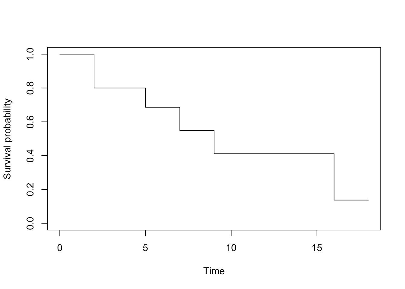
To draw this survival curve, remember that:
- the x-axis corresponds to the
timevariable in the initial dataset, and - the y-axis corresponds to the survival probabilities found above.
In R
We now compare our results with the results found in R.
We first create the dataset with the time and event variables:
# create dataset
dat <- data.frame(
  time = c(3, 5, 7, 2, 18, 16, 2, 9, 16, 5),
  event = c(0, 1, 1, 1, 0, 1, 1, 1, 1, 0)
)
We then run the Kaplan-Meier estimator with the survfit() and Surv() functions:
# KM
library(survival)

km <- survfit(Surv(time, event) ~ 1,
  data = dat
)
Notice that the Surv() function accepts two arguments:
- the
timevariable, and - the
eventvariable.
The ~ 1 in the survfit() function indicates that we estimate the Kaplan-Meier without any grouping. See more on this later in the post.
Finally, we display the results and draw the Kaplan-Meier plot:
# results
summary(km)
## Call: survfit(formula = Surv(time, event) ~ 1, data = dat)
##
## time n.risk n.event survival std.err lower 95% CI upper 95% CI
## 2 10 2 0.800 0.126 0.5868 1.000
## 5 7 1 0.686 0.151 0.4447 1.000
## 7 5 1 0.549 0.172 0.2963 1.000
## 9 4 1 0.411 0.176 0.1782 0.950
## 16 3 2 0.137 0.126 0.0225 0.834# plot
plot(km,
xlab = "Time",
ylab = "Survival probability",
conf.int = FALSE
)
The survival probabilities can be found in the survival column. Remark that results by hand and in R are similar (any difference with the results by hand is due to rounding).
Alternatively, we can use the ggsurvplot() function within the {survminer} package:
library(survminer)

# plot
ggsurvplot(km,
  conf.int = FALSE,
  legend = "none"
)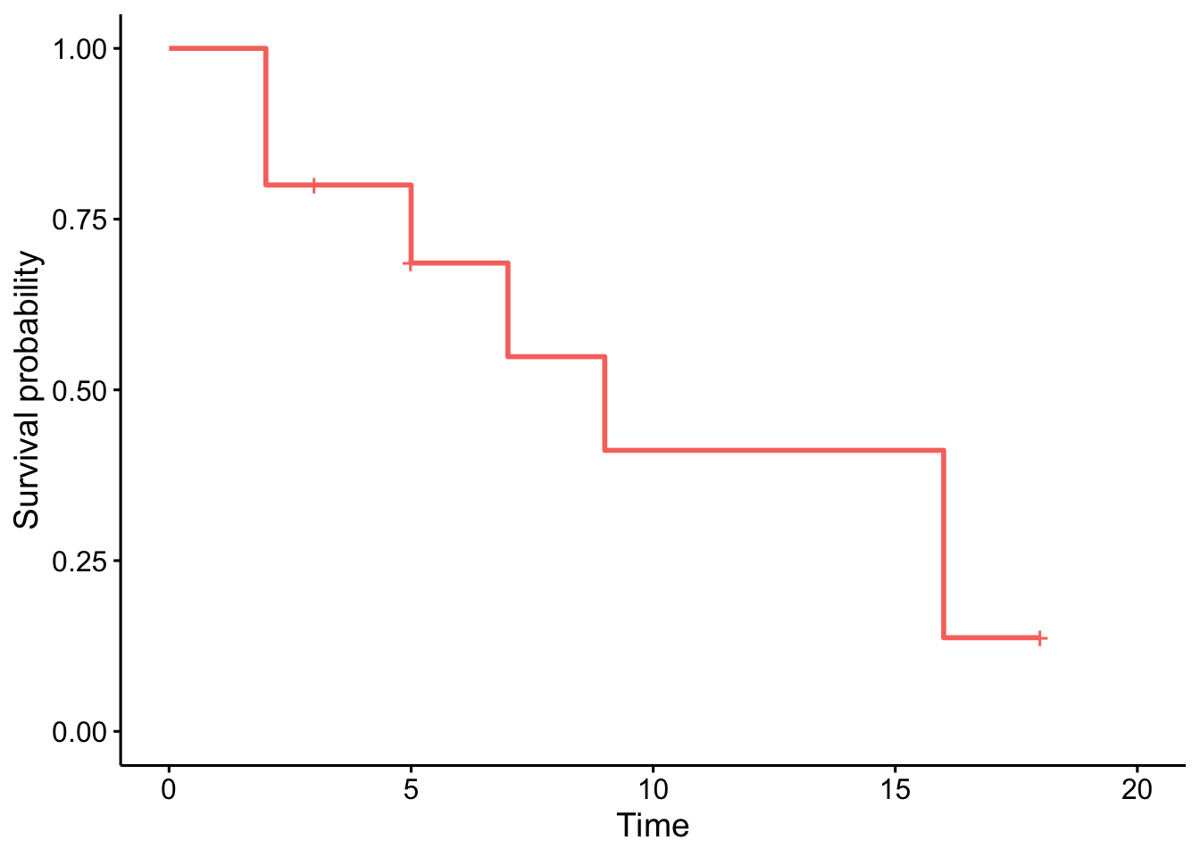
Note that the crosses on the survival curve denote the censored observations.
The advantage with the ggsurvplot() function is that it is easy to draw the median survival directly on the plot:3
ggsurvplot(km,
  conf.int = FALSE,
  surv.median.line = "hv",
  legend = "none"
)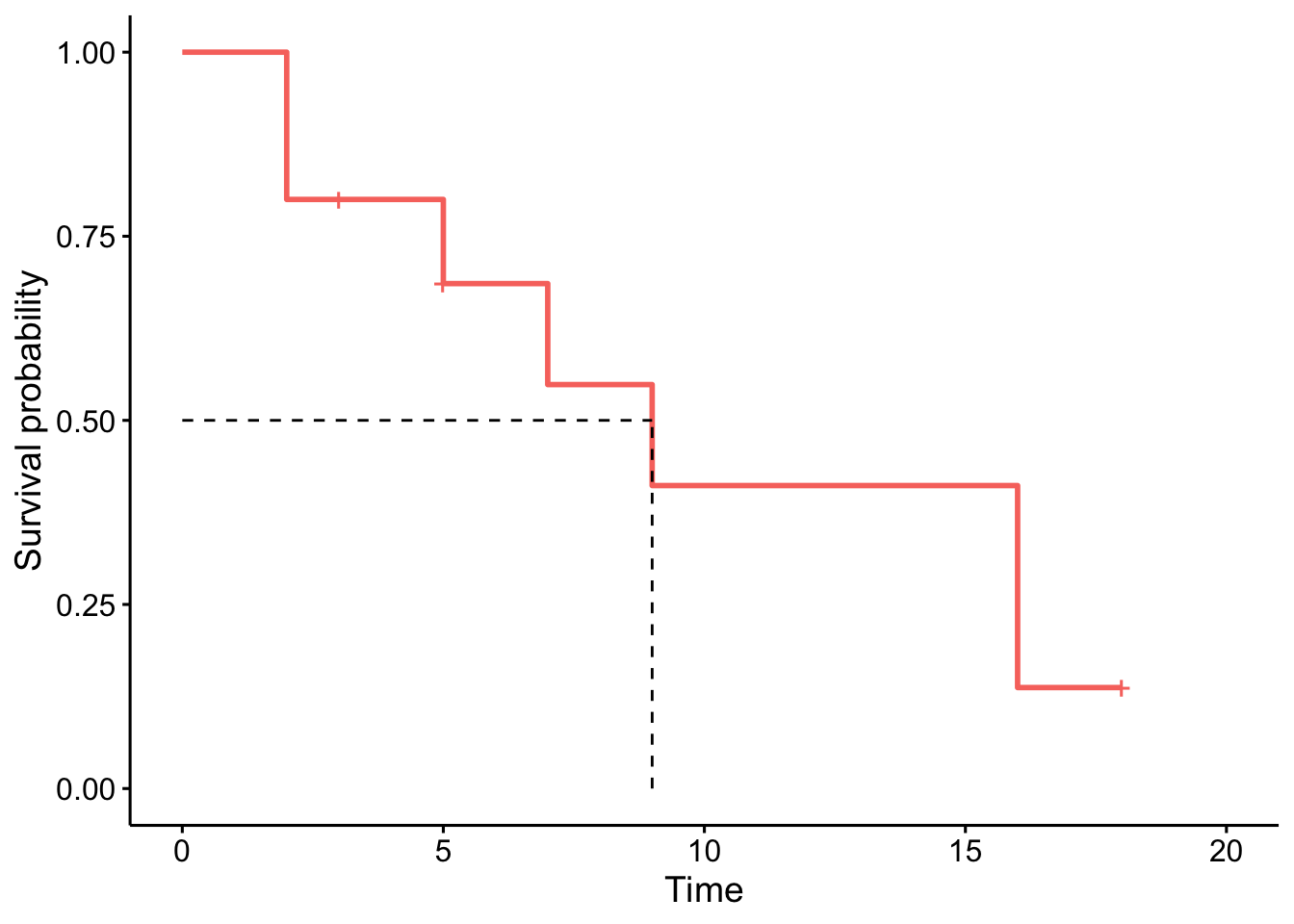
To find the median survival:4
summary(km)$table["median"]## median
## 9# or more simply
km## Call: survfit(formula = Surv(time, event) ~ 1, data = dat)
##
## n events median 0.95LCL 0.95UCL
## [1,] 10 7 9 5 NASuppose that the event of interest is death:
- At time zero, the survival probability is 1 (100% of the subjects are alive).
- The median indicates that the median survival time is 9 years.5 This is the time at which the survival \(S(t)\) is 50%. In other words, is the time after which half of the subjects are expected to have died.
- From the plot, we also see that \(S(5) = P(T > 5 \text{ years}) =\) Probability of survival of more than 5 years for these subjects = 75%. This means that 75% of all subjects survive longer than 5 years, and that 25% of all subjects die within the first 5 years.
For the sake of completeness, let’s do another example with a much larger dataset; the tongue dataset within the {KMsurv} package.6
# load data
library(KMsurv)
data(tongue)

# preview data
head(tongue)
## type time delta
## 1 1 1 1
## 2 1 3 1
## 3 1 3 1
## 4 1 4 1
## 5 1 10 1
## 6 1 13 1typeis the tumor DNA profile (1 = aneuploid tumor, 2 = diploid tumor)timeis the time to death or on-study time (in weeks)deltais the death indicator (0 = alive, 1 = dead)
For this example, we focus on the aneuploid type:
anaploid <- subset(tongue, type == 1)We can now plot the estimated survival function and estimate the median time to death. Since it is an estimator, we can also construct a confidence interval for the estimated survival at each time \(t\) and for the estimated median survival time.7
# results
fit <- survfit(Surv(time, delta) ~ 1,
  data = anaploid,
  conf.type = "log-log"
)

fit
## Call: survfit(formula = Surv(time, delta) ~ 1, data = anaploid, conf.type = "log-log")
##
## n events median 0.95LCL 0.95UCL
## [1,] 52 31 93 65 157# plot
ggsurvplot(fit,
surv.median.line = "hv",
legend = "none"
)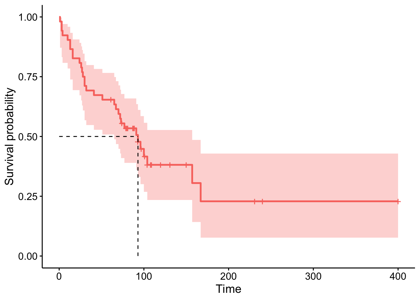
The median survival time is estimated to be 93 weeks, with a 95% confidence interval between 65 and 157 weeks.
Kaplan-Meier curves can be seen as descriptive statistics for survival data. We now focus on the second branch of statistics, hypothesis testing which allows to draw conclusions on the population based on a sample (see a quick reminder about the difference between population and sample if you need).
Hypothesis testing
Hypothesis testing in the field of survival analysis mostly concerns:
- The hazard function of one population: in this case we test whether a censored sample comes from a population with a known hazard function \(h_0(t)\). For example, we may be interested to compare survival in a sample of patients to the survival in the overall population (derived from the life tables).
- The comparison of the hazard function of two or more populations: in this case we are interested in assessing whether there are differences in survival among different groups of subjects. For example:
- 2 groups: we are interested in comparing survival for female and male colon cancer patients
- 3 groups or more: we are interested in comparing survival for melanoma cancer patients according to their treatments (with treatments A, B and C for example)8
Log-rank test
In this article, we focus on comparing survival between two groups using the log-rank test (also known as Mantel-Cox test). This test is the most common hypothesis test to compare survival between two groups.
The intuition behind the test is that if the two groups have different hazard rates, the two survival curves (so their slopes) will differ. More precisely, the log-rank test compares the observed number of events in each group to what would be expected if the survival curves were identical (i.e., if the null hypothesis were true).
Note that, as for the Kaplan-Meier estimator, the log-rank test is a nonparametric test, which makes no assumptions about the survival distributions.
For this example, consider the following dataset:
##    patient group time event
## 1        1     1  4.1     1
## 2        2     1  7.8     0
## 3        3     1 10.0     1
## 4        4     1 10.0     1
## 5        5     1 12.3     0
## 6        6     1 17.2     1
## 7        7     2  9.7     1
## 8        8     2 10.0     1
## 9        9     2 11.1     0
## 10      10     2 13.1     0
## 11      11     2 19.7     1
## 12      12     2 24.1     0
where:
patientis the patient’s identifiergroupis the group (group 1 or 2)timeis the time to death (in years)9eventis the event status (0 = censored, 1 = death)
Suppose we are interested in comparing group 1 and 2 in terms of survival, that is, we compare survival curves between the 2 groups:
- \(H_0 : S_1(t) = S_2(t)\) for all \(t\)
- \(H_1 : S_1(t) \ne S_2(t)\) for some \(t\)
It is a statistical test, so if the \(p\)-value < \(\alpha\) (usually 0.05), we reject the null hypothesis and we conclude that survival (or the time to event) is significantly different between the two groups considered.
To perform the log-rank test, the following test statistic will be useful:
\[\begin{eqnarray} U &=& \sum_{j=1}^r w(y_{(j)})\left(O_j - E_j\right) \\ &=& \sum_{j=1}^r w(y_{(j)})\left( d_{(j)1} - \frac{d_{(j)}R_{(j)1}}{R_{(j)}}\right) \end{eqnarray}\]
with \(U^{obs} = \frac{U}{\sqrt{Var(U)}} \sim N(0,1)\) and10
\[\begin{eqnarray} Var(U) &=& \sum_{j=1}^r w^2(y_{(j)}) \frac{N_{(j)}}{ D_{(j)} }\\ &=& \sum_{j=1}^r w^2(y_{(j)}) \frac{ d_{(j)} \frac{R_{(j)1}}{R_{(j)} } \left( 1 - \frac{R_{(j)1}}{R_{(j)} } \right) \left( R_{(j)} - d_{(j)}\right) }{ R_{(j)} - 1 } \end{eqnarray}\]
By hand
As for the Kaplan-Meier estimator by hand, it is best to also fill in a table for the log-rank test by hand.
Let’s present the final table and comment below on how to fill it, column by column:
| \(j\) | \(y_{(j)}\) | \(d_{(j)1}\) | \(R_{(j)1}\) | \(d_{(j)2}\) | \(R_{(j)2}\) | \(d_{(j)}\) | \(R_{(j)}\) | \(E_{j}\) | \(O_{j}\) | \(O_{j} - E_{j}\) | \(N_{(j)}\) | \(D_{(j)}\) | \(N_{(j)}/D_{(j)}\) |
|---|---|---|---|---|---|---|---|---|---|---|---|---|---|
| 1 | 4.1 | 1 | 6 | 0 | 6 | 1 | 12 | 0.5 | 1 | 0.5 | 2.75 | 11 | 0.25 |
| 2 | 9.7 | 0 | 4 | 1 | 6 | 1 | 10 | 0.4 | 0 | -0.4 | 2.16 | 9 | 0.24 |
| 3 | 10 | 2 | 4 | 1 | 5 | 3 | 9 | 1.333 | 2 | 0.667 | 4.44 | 8 | 0.555 |
| 4 | 17.2 | 1 | 1 | 0 | 2 | 1 | 3 | 0.333 | 1 | 0.667 | 0.44 | 2 | 0.22 |
| 5 | 19.7 | 0 | 0 | 1 | 2 | 1 | 2 | 0 | 0 | 0 | 0.00 | 1 | 0.00 |
| \(Total\) | 4 | 3 | 7 | 2.566 | 1.433 | 1.265 |
Column \(j\) is the number of distinct event times. We see that there are 5 (ignoring censored observations), so we write 1 to 5 in the table.
Column \(y_{(j)}\) is the ordered distinct event times:
4.1, 9.7, 10, 17.2 and 19.7
Column \(d_{(j)1}\) is the number of observations for each distinct event time, for group 1:
## time
##  4.1   10 17.2
##    1    2    1
When there is no event, we simply write 0 in the table.
Column \(R_{(j)1}\) is the remaining number of patients at risk, for group 1. For this, the distribution of time (censored and not censored, for group 1) is useful:
## time
##  4.1  7.8   10 12.3 17.2
##    1    1    2    1    1
We see that:
- At the beginning, there are 6 patients
- Before time 9.7, there are 4 patients left (6 - 1 who had the event at time 4.1 - 1 who was censored at time 7.8)
- Before time 10, there are 4 patients left (6 - 2)
- Before time 17.2, there are 1 patient left (6 - 5)
- Before time 19.7, there are 0 patient left (6 - 6)
Columns \(d_{(j)2}\) and \(R_{(j)2}\) follow the same principle, but for group 2 this time. So we have, respectively for \(d_{(j)2}\) and \(R_{(j)2}\):
## time
##  9.7   10 19.7
##    1    1    1
## time
## 9.7 10 11.1 13.1 19.7 24.1
## 1 1 1 1 1 1Columns \(d_{(j)}\) and \(R_{(j)}\) also follow the same principle, but this time considering both groups. So we have, respectively for \(d_{(j)}\) and \(R_{(j)}\):
## time
##  4.1  9.7   10 17.2 19.7
##    1    1    3    1    1
## time
## 4.1 7.8 9.7 10 11.1 12.3 13.1 17.2 19.7 24.1
## 1 1 1 3 1 1 1 1 1 1Column \(E_{j}\) is the expected number of events in the first group assuming that \(h_1 \equiv h_2\). It is obtained as follows
\[ E_{j} = \frac{d_{(j)}R_{(j)1}}{R_{(j)}}\]
Column \(O_{j}\) is the observed number of events in the first group, so it is equal to the \(d_{(j)1}\) column.
Column \(O_{j} - E_{j}\) is straightforward.
Column \(N_{(j)}\) is defined as follows
\[N_{(j)} = d_{(j)} \frac{R_{(j)1}}{R_{(j)} } \left( 1 - \frac{R_{(j)1}}{R_{(j)} } \right) \left( R_{(j)} - d_{(j)}\right)\]
Column \(D_{(j)}\) is \(R_{(j)} - 1\).
Column \(N_{(j)}/D_{(j)}\) is straightforward.
Since \(w(y_{(j)}) = w^2(y_{(j)}) = 1\) for a log-rank test, we have11
\[ U^{obs} = \frac{U}{\sqrt{Var(U)}} = \frac{1.434}{\sqrt{1.265}} = 1.275.\]
We reject \(H_0\) if \(|U^{obs}|>z_{1-\alpha/2}\), so at the 5% significance level we reject \(H_0\) if \(|U^{obs}|>z_{0.975}=1.96\).
We have \(|U^{obs}| = 1.275 < z_{0.975}=1.96\). Hence, at the 5% significance level we do not reject \(H_0\). This means that, based on the data, we are not able to conclude that survival is different between the two groups (which is equivalent than saying that we do not reject the hypothesis that survival is equal between the two groups).
If you are interested in computing the \(p\)-value:
\(p\)-value \(= 2\times P(Z>1.275) = 2 \times 0.101 = 0.202 > 0.05\).
In R
We now compare our results in R with the survdiff() function:
dat <- data.frame(
  group = c(rep(1, 6), rep(2, 6)),
  time = c(4.1, 7.8, 10, 10, 12.3, 17.2, 9.7, 10, 11.1, 13.1, 19.7, 24.1),
  event = c(1, 0, 1, 1, 0, 1, 1, 1, 0, 0, 1, 0)
)

dat
## group time event
## 1 1 4.1 1
## 2 1 7.8 0
## 3 1 10.0 1
## 4 1 10.0 1
## 5 1 12.3 0
## 6 1 17.2 1
## 7 2 9.7 1
## 8 2 10.0 1
## 9 2 11.1 0
## 10 2 13.1 0
## 11 2 19.7 1
## 12 2 24.1 0survdiff(Surv(time, event) ~ group,
data = dat
)## Call:
## survdiff(formula = Surv(time, event) ~ group, data = dat)
##
## N Observed Expected (O-E)^2/E (O-E)^2/V
## group=1 6 4 2.57 0.800 1.62
## group=2 6 3 4.43 0.463 1.62
##
## Chisq= 1.6 on 1 degrees of freedom, p= 0.2Alternatively, we can use the ggsurvplot() function to draw the survival curves and perform the log-rank test at the same time:
fit <- survfit(Surv(time, event) ~ group, data = dat)

ggsurvplot(fit,
  pval = TRUE,
  pval.method = TRUE
)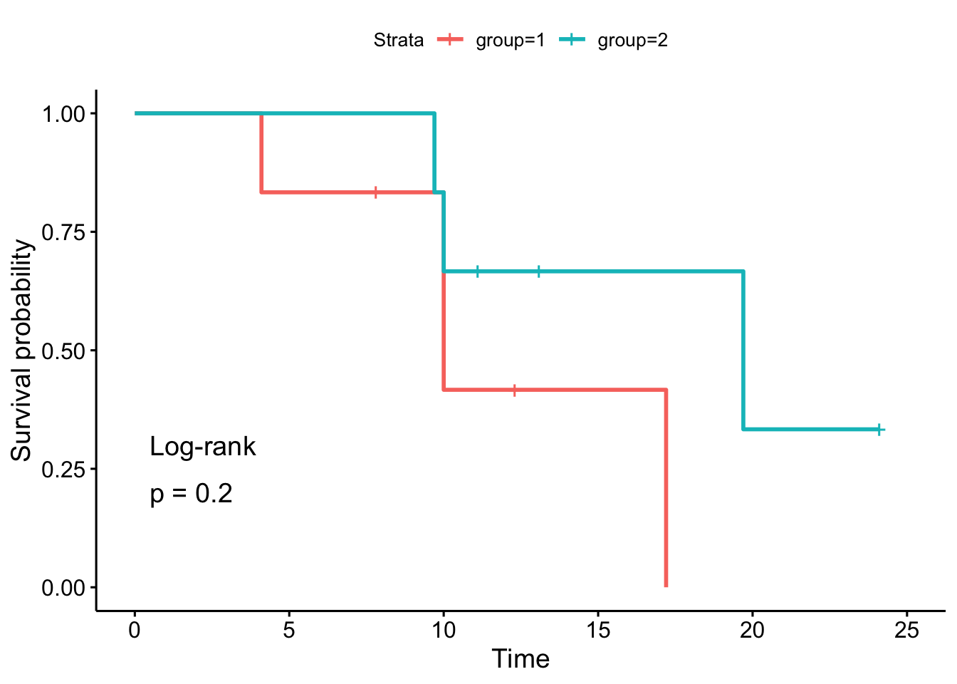
As we can see, the \(p\)-values and the conclusions are the same (any difference with the results by hand is due to rounding).
As for the Kaplan-Meier estimation, we do another example on a larger dataset. Consider the data on the times until staphylococcus infection of burn patients, also available in the {KMsurv}:12
# load data
data(burn)

# preview data
head(burn)
## Obs Z1 Z2 Z3 Z4 Z5 Z6 Z7 Z8 Z9 Z10 Z11 T1 D1 T2 D2 T3 D3
## 1 1 0 0 0 15 0 0 1 1 0 0 2 12 0 12 0 12 0
## 2 2 0 0 1 20 0 0 1 0 0 0 4 9 0 9 0 9 0
## 3 3 0 0 1 15 0 0 0 1 1 0 2 13 0 13 0 7 1
## 4 4 0 0 0 20 1 0 1 0 0 0 2 11 1 29 0 29 0
## 5 5 0 0 1 70 1 1 1 1 0 0 2 28 1 31 0 4 1
## 6 6 0 0 1 20 1 0 1 0 0 0 4 11 0 11 0 8 1Using the log-rank test, we want to test the hypothesis of difference in the time to staphylococcus infection (T3 variable) between patients whose burns were cared for with a routine bathing care method (Z1 = 0) versus those whose body cleansing was initially performed using 4% chlorhexidine gluconate (Z1 = 1). The event indicator is in variable D3.
For this test, we use a two-sided alternative and a 5% significance level.
# fit
fit <- survfit(Surv(T3, D3) ~ Z1, data = burn)

# plot with log-rank test
ggsurvplot(fit,
  pval = TRUE,
  pval.method = TRUE
)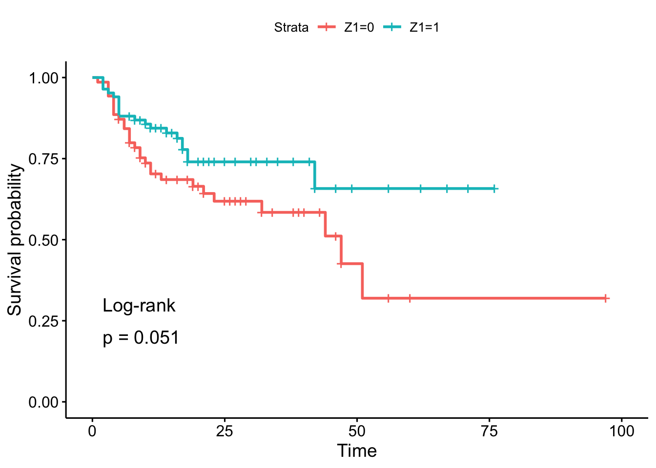
In the sample, it seems that the time to infection for patients with routine bathing (Z1 = 0) is smaller than for patients with body cleansing (Z1 = 1). This is the case because the percentage of patients who have not experienced the infection decreases more quickly, so the hazard rate is greater.
However, this conclusion cannot be generalized to the population without performing a sound statistical test. And based on the result of the log-rank test, we do not reject the hypothesis that time to infection is the same between the two groups of patients (\(p\)-value = 0.051).
To go further
In this article, we have presented what is survival analysis, when, why and how to use it. We discussed about censoring and survival curves. We showed how to estimate the survival function via the Kaplan-Meier estimator and how to test survival between two groups via the log-rank test. We illustrated these approaches both by hand and in R.
As you noticed, we did not show how to model survival data. There are several regression models that can be applied to survival data, the most common one being the semiparametric Cox Proportional Hazards model (1972). It originated from the medical area to investigate and assess the relationship between the survival times of patients and their corresponding predictor variables.
We have seen that the Kaplan-Meier estimator is useful to visualize survival between groups and the log-rank test to test whether survival significantly differs between groups (so both approaches use a categorical variable as predictor). However, it does not work well for assessing the effect of quantitative predictor. The Cox model has the advantage that it works for both quantitative as well as for categorical predictors, and for several risk factors at the same time (so it can model the effect of multiple variables at once).
With the Cox model, we model the impact of different factors \(X_1, X_2, \ldots, X_q\) on survival via their impact on the hazard function:
\[h(t|\textbf{X}) = h_0 (t) exp(\beta_1 X_1 + \beta_2 X_2 + \cdots + \beta_q X_q),\]
where:
- \(h(t|\textbf{X})\) is the instantaneous death rate conditional on having survived up to time \(t\).
- \(h_0 (t)\) is the population-level baseline hazard – the underlying hazard function. It describes how the average person’s risk evolves over time.
- \(exp(\beta_1 X_1 + \beta_2 X_2 + \cdots + \beta_q X_q)\) describes how covariates affect the hazard. In particular, a unit increase in \(x_i\) leads to an increase of the hazard by a factor of \(\exp(\beta_i)\).
This post aimed at presenting the introductory concepts in survival analysis, so this model will be developed in another post. In the meantime, if you would like to learn more about modeling survival data (thanks to the Cox model and other models), see this post from Joseph Rickert.
Thanks for reading.
As always, if you have a question or a suggestion related to the topic covered in this article, please add it as a comment so other readers can benefit from the discussion.
References
Note that in survival analysis, the precision of the estimators (and the power of the tests) does not depend on the number of patients but on the number of events. So it is best to have many observations where the event does occur for the analyses to be effective. Here we work on a small sample for the sake of illustration.↩︎
Note that the
timevariable can be expressed in other units, such as seconds, days, weeks, months, etc.↩︎Median is preferred over mean in survival analysis because survival functions are often skewed to the right. The mean is often influenced by outliers, whereas the median is not. See a discussion comparing the two in this section.↩︎
Note that if the survival curve does not cross 50% (because survival is greater than 50% at the last time point), then the median survival cannot be computed and is simply undefined.↩︎
Note that the median survival is expressed in the same unit than the unit of the
timevariable in the initial dataset. So if the time unit was months, the median survival time would be 9 months.↩︎More information about the dataset can be found on CRAN or with
?tongue.↩︎See the reason we use
log-logfor the confidence interval in this thread.↩︎Note that if the groups to compare have a natural ordering (such as the educational level; none, low, medium, high), tests that take it into consideration have more power to detect significant effects. These tests are referred as tests for trend.↩︎
Remember that the time unit can be different than years.↩︎
This is the case for large samples. The example described here does not meet this condition, but we still show it as an illustration.↩︎
Note that other weights can be considered, but this is beyond the scope of this article.↩︎
More information about the dataset can be found on CRAN or with
?burn.↩︎
Liked this post?
- Get updates every time a new article is published (no spam and unsubscribe anytime)
- Support the blog
- Share on:


