
Web scraping in R

Note: This post has been written in collaboration with Pietro Zanotta.
Introduction
Almost anyone is familiar with web pages (otherwise you would not be here), but what if we tell you that how you see a site is different from how Google or your browser does?
In fact, when you type any site address in your browser, your browser will download and render the page for you, but for rendering the page it needs some instructions.
There are 3 types of instructions:
- HTML: describes a web page’s infrastructure;
- CSS: defines the appearance of a site;
- JavaScript: decides the behavior of the page.
Web scraping is the art of extracting information from the HTML, CSS and Javascript lines of code. The term usually refers to an automated process, which is less error-prone and faster than gathering data by hand.
It is important to note that web scraping can raise ethical concerns, as it involves accessing and using data from websites without the explicit permission of the website owner. It is a good practice to respect the terms of use for a website, and to seek written permission before scraping large amounts of data.
This article aims to cover the basics of how to do web scraping in R. We will conclude by creating a database on Formula 1 drivers from Wikipedia.
Note that this article doesn’t want to be exhaustive on topic. To learn more, see this section.
HTML and CSS
Before starting it is important to have a basic knowledge of HTML and CSS. This section aims to briefly explain how HTML and CSS work, to learn more we leave you some resources at the bottom of this article.
Feel free to skip this section if you already are knowledgeable in this topic.
Starting from HTML, an HTML file looks like the following piece of code.
<!DOCTYPE html>
<html lang="en">
<body>

<h1 href="https://en.wikipedia.org/wiki/Carl_Friedrich_Gauss"> Carl Friedrich Gauss</h1>
<h2> Biography </h2>
<p> Johann Carl Friedrich Gauss was born on 30 April 1777 in Brunswick. </p>
<h2> Profession </h2>
<p> Gauss is considered as one of the greatest mathematician, statistician and physicist of all time. </p>

</body>
</html>
Those instructions produce the following:
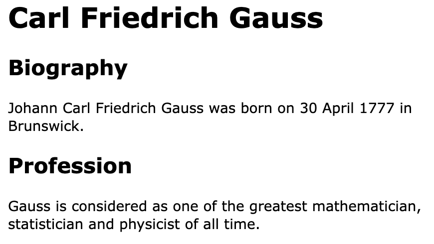
As you read above, HTML is used to describe the infrastructure of a web page, for example we may want to define the headings, the paragraphs, etc.
This infrastructure is represented by what are called tags (for example <h1>...</h1> or <p>...</p> are tags). Tags are the core of an HTML document as they represent the nature of what is inside the tag (for example h1 stands for heading 1). It is important to observe that there are two types of tags:
- starting tags (e.g.
<h1>) - ending tags (e.g.
</h1>)
This is what allows to nest different tags.
Tags can also have attributes, for example in <h1 href="https://en.wikipedia.org/wiki/Carl_Friedrich_Gauss">Carl Friedrich Gauss</h1>, href is an attribute of the tag h1 that specifies an URL.
As the output of the above HTML code is not super elegant, CSS is used to style the final website. For example CSS is used to define the font, the color, the size, the spacing and many more features of a website.
What is important for this article are CSS selectors, which are patterns used to select elements. The most important is the .class selector, which selects all elements with the same class. For example the .xyz selector selects all elements with class="xyz".
Web scraping vs. APIs
Going back to web scraping, you may know that APIs are another way to access data from websites and online services.
In fact an API is a set of rules and protocols that allows two different software systems to communicate with each other. When a website or online service provides an API, it means that they have made it possible for developers to access their data in a structured and controlled way.
Why does web scraping exist if APIs are so powerful and do exactly the same work?
The main difference between web scraping and using APIs is that APIs are typically provided by the website or service to allow access to their data, while web scraping involves accessing data without the explicit permission of the website owner.
This means that using APIs is generally considered more ethical than web scraping, as it is done with the explicit permission of the website or service.
However, there are also some limitations to using APIs:
- many APIs have rate limits, which means that they will only allow a certain number of requests to be made within a certain time period, i.e. you may not access large amounts of data;
- not all websites or online services provide APIs, which means the only way to access their data is via web scraping.
Web scraping in R
There are several packages for web scraping in R, every package has its strengths and limitations. We will cover only the rvest package since it is the most used.
To get started with web scraping in R you will first need R and RStudio installed (if needed, see here). Once you have R and RStudio installed, you need to install the rvest package:
install.packages("rvest")rvest
Inspired by beautiful soup and RoboBrowser (two Python libraries for web scraping), rvest has a similar syntax, which makes it the most eligible package for those who come from Python.
rvest provides functions to access a web page and specific elements using CSS selectors and XPath. The library is a part of the Tidyverse collection of packages, i.e. it shares some coding conventions (e.g. the pipes) with other libraries as tibble and ggplot2.
Before the real scraping it is necessary to load the rvest package:
library(rvest)Now that everything is settled down, we can start the web scraping operation, which is usually made in 3 steps:
- HTTP GET request
- Parsing HTML content
- Getting HTML element attributes
These steps are detailed in the following sections.
HTTP GET request
The HTTP GET method is a method used to send a server a question to get certain data and information. It is important to notice that this method does not change the state of the server.
To send a GET request we need the link (as a character) to the page we want to scrape:
link <- "https://www.nytimes.com/"Sending the request to the page is simple, rvest provides the read_html function, which returns an object of html_document type:
NYT_page <- read_html(link)

NYT_page
## {html_document}
## <html lang="en" class=" nytapp-vi-homepage tpl-always-light" xmlns:og="http://opengraphprotocol.org/schema/">
## [1] <head>\n<meta http-equiv="Content-Type" content="text/html; charset=UTF-8 ...
## [2] <body>\n \n <div id="app">\n<link rel="preload" as="image" href="/v ...Parsing HTML content
As we saw in the last chunk of code, NYT_page contains the raw HTML code, which is not so easily readable.
In order to make it readable from R it has to be parsed, which means generating a Document Object Model (DOM) from the raw HTML. DOM is what connects scripts and web pages by representing the structure of a document in memory. If you retrieve the HTTP request using Node.js, you can give the raw HTML response to R for parsing and further analysis.
rvest provides 2 ways to select HTML elements:
- XPath
- CSS selectors
Selecting elements with rvest is simple, for XPath we use the following syntax:
NYT_page %>%
  html_elements(xpath = "")
while for CSS elector we need:
NYT_page %>%
  html_elements(css = "")
CSS selector
Suppose that for a project you need the summaries of the articles of the NYT (note that what is in the following picture is not what you see in the New York Times web page).
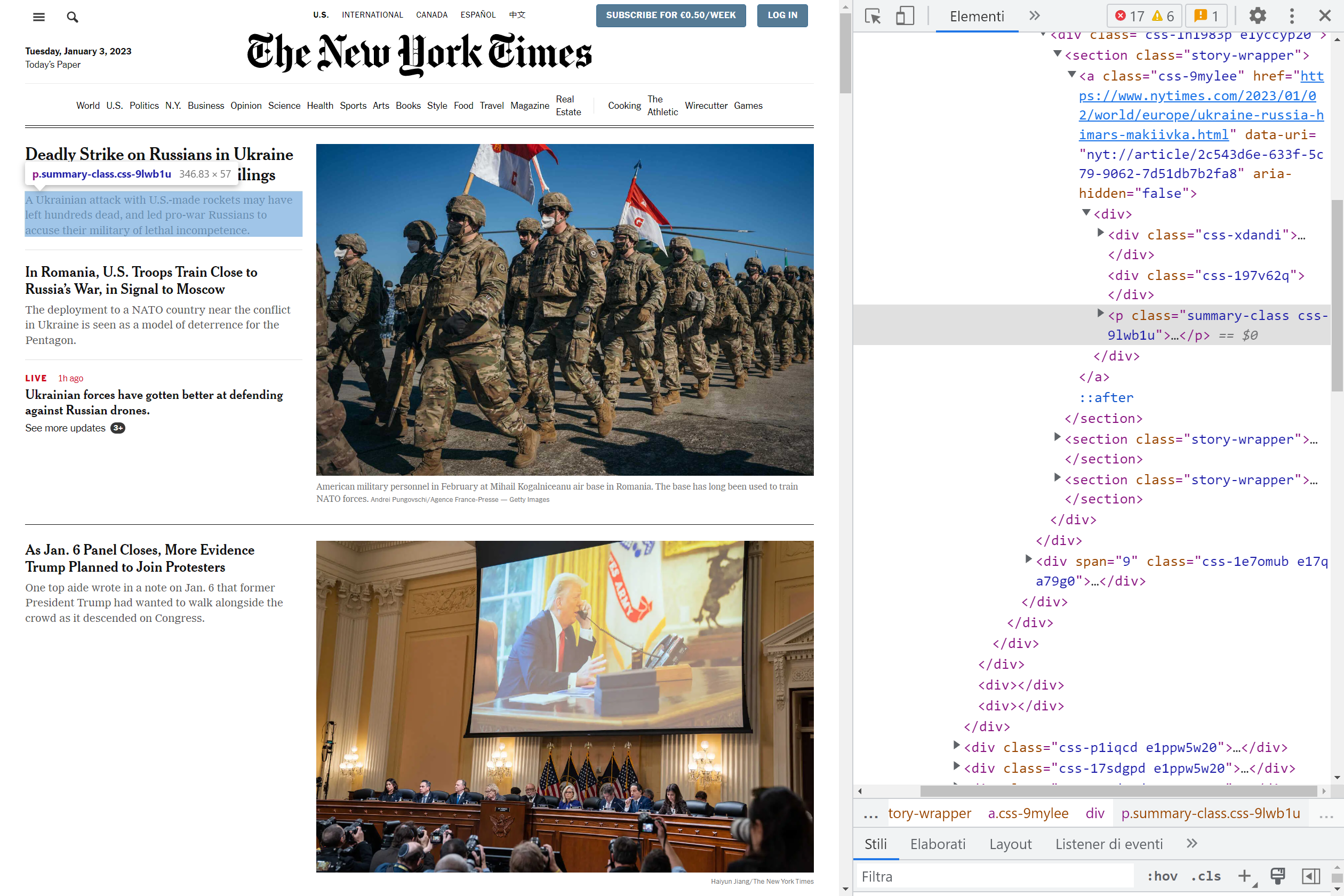
Searching in the HTML code, it is not that complex to find <p class="summary-class">, which is the markup of what we are looking for. To parse the HTML using this selector we use the html_element function:
summaries_css <- NYT_page %>%
  html_elements(css = ".summary-class")

head(summaries_css)
## {xml_nodeset (6)}
## [1] <p class="summary-class css-crclbt">At least 18 were killed in Kyiv, offi ...
## [2] <p class="summary-class css-1vqq9lj">Long-delayed funeral ceremonies for ...
## [3] <p class="summary-class css-1vqq9lj">Senior U.S. officials have said Iran ...
## [4] <p class="summary-class css-1vqq9lj">One of England’s greatest World Cup ...
## [5] <p class="summary-class css-1vqq9lj">America’s 2-0 win over Bosnia and He ...
## [6] <p class="summary-class css-1vqq9lj">Some data suggest artificial intelli ...The easiest way to obtain a CSS selector is opening the inspect mode, find the element you desire and right click on it. Then click on copy and copy selector.
XPath
Parsing with XPath is similar to parsing using selectors. In fact, we just need to repeat what we did above using XPath of the element of interest. Moreover, obtaining an element’s XPath is not different form selector: inspector mode -> right click on element of interest -> copy -> copy XPath.
Repeating what we did above with XPath:
summaries_xpath <- NYT_page %>%
  html_elements(xpath = "//*[contains(@class, 'summary-class')]")

head(summaries_xpath)
## {xml_nodeset (6)}
## [1] <p class="summary-class css-crclbt">At least 18 were killed in Kyiv, offi ...
## [2] <p class="summary-class css-1vqq9lj">Long-delayed funeral ceremonies for ...
## [3] <p class="summary-class css-1vqq9lj">Senior U.S. officials have said Iran ...
## [4] <p class="summary-class css-1vqq9lj">One of England’s greatest World Cup ...
## [5] <p class="summary-class css-1vqq9lj">America’s 2-0 win over Bosnia and He ...
## [6] <p class="summary-class css-1vqq9lj">Some data suggest artificial intelli ...Obviously the data we collected with CSS selector and XPath are exactly the same.
Getting attributes
Since the chunk of code above collect all the elements p with the class summary, we render all the elements of NYT_summary_css as a text using the html_text function:
NYT_summaries_css <- html_text(summaries_css)
NYT_summaries_xpath <- html_text(summaries_xpath)
We only print some of them:
head(NYT_summaries_css)## [1] "At least 18 were killed in Kyiv, officials said. Ukraine’s president had warned of a “massive strike” as his country’s forces hit deeper into Russian territory."
## [2] "Long-delayed funeral ceremonies for Ayatollah Ali Khamenei, killed during U.S.-Israeli strikes at the war’s outset, are set to begin Friday."
## [3] "Senior U.S. officials have said Iran would be richly rewarded for changing its stance on America. But Tehran has rejected such a bargain in the past."
## [4] "One of England’s greatest World Cup moments unfolded on Wednesday, a columnist for The Athletic writes."
## [5] "America’s 2-0 win over Bosnia and Herzegovina sets up a round-of-16 showdown with Belgium."
## [6] "Some data suggest artificial intelligence is already causing job losses. Other sources show the opposite. Why is it so hard to figure out what’s going on?"A real application of web scraping in R

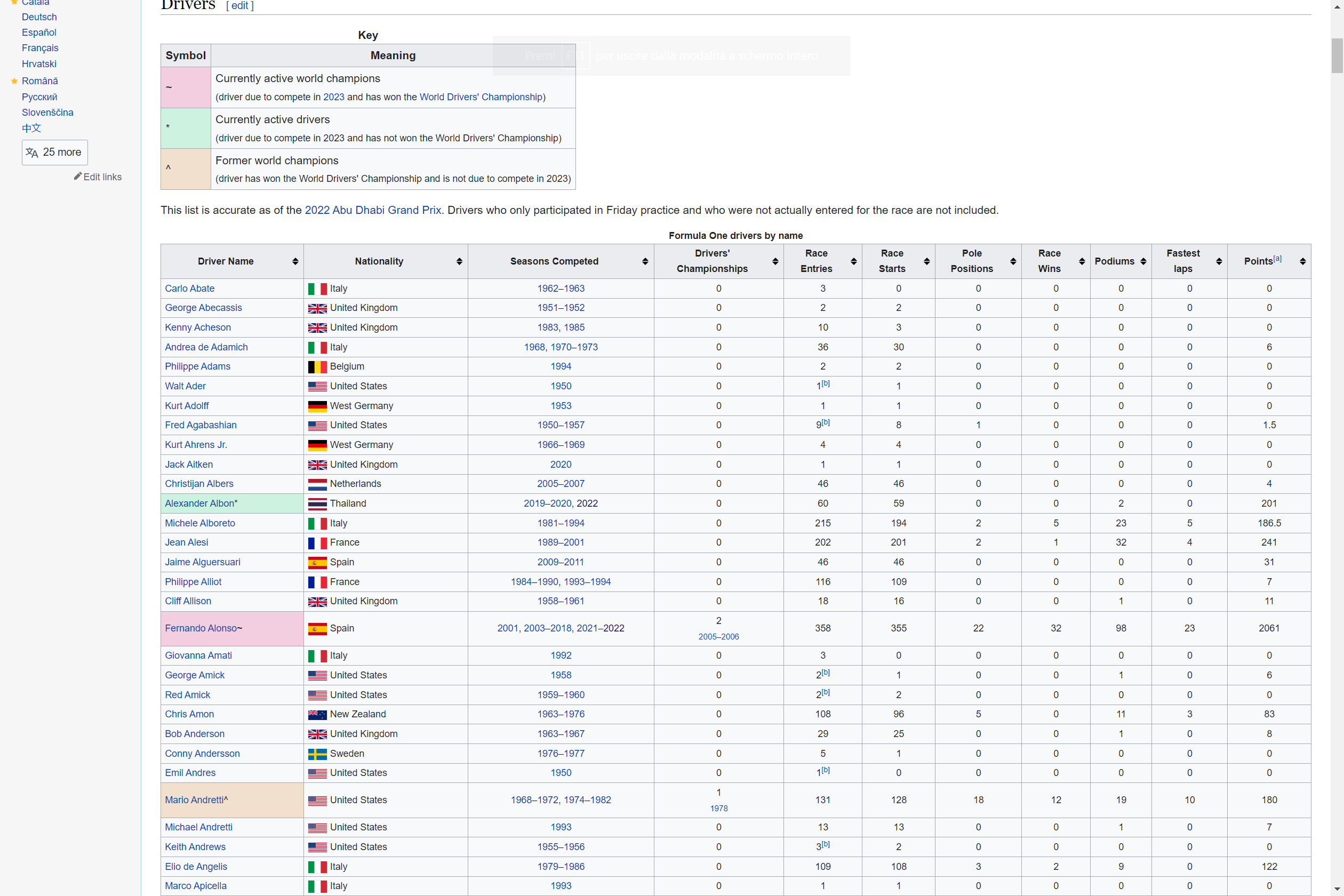
To conclude this brief introduction to web scraping we want to use the rvest package in a real word application of web scraping. The goal is to scrape data from Formula 1 Wikipedia’s voice and create a CSV file containing the name, the nationality, the number of podiums and some other statistics for every pilot.
The table we are going to scrape is the following:
If you haven’t done so, you need to install the rvest package:
install.packages("rvest")and then load it:
library(rvest)HTTP GET request
The GET request is the easiest part of scraping, we just need the following line of code:
link <- "https://en.wikipedia.org/wiki/List_of_Formula_One_drivers"Parsing HTML content and getting attributes
Again we repeat what we did before with the NYT example:
page <- read_html(link)Searching in the HTML code we find that the table is a table element with the sortable attribute:
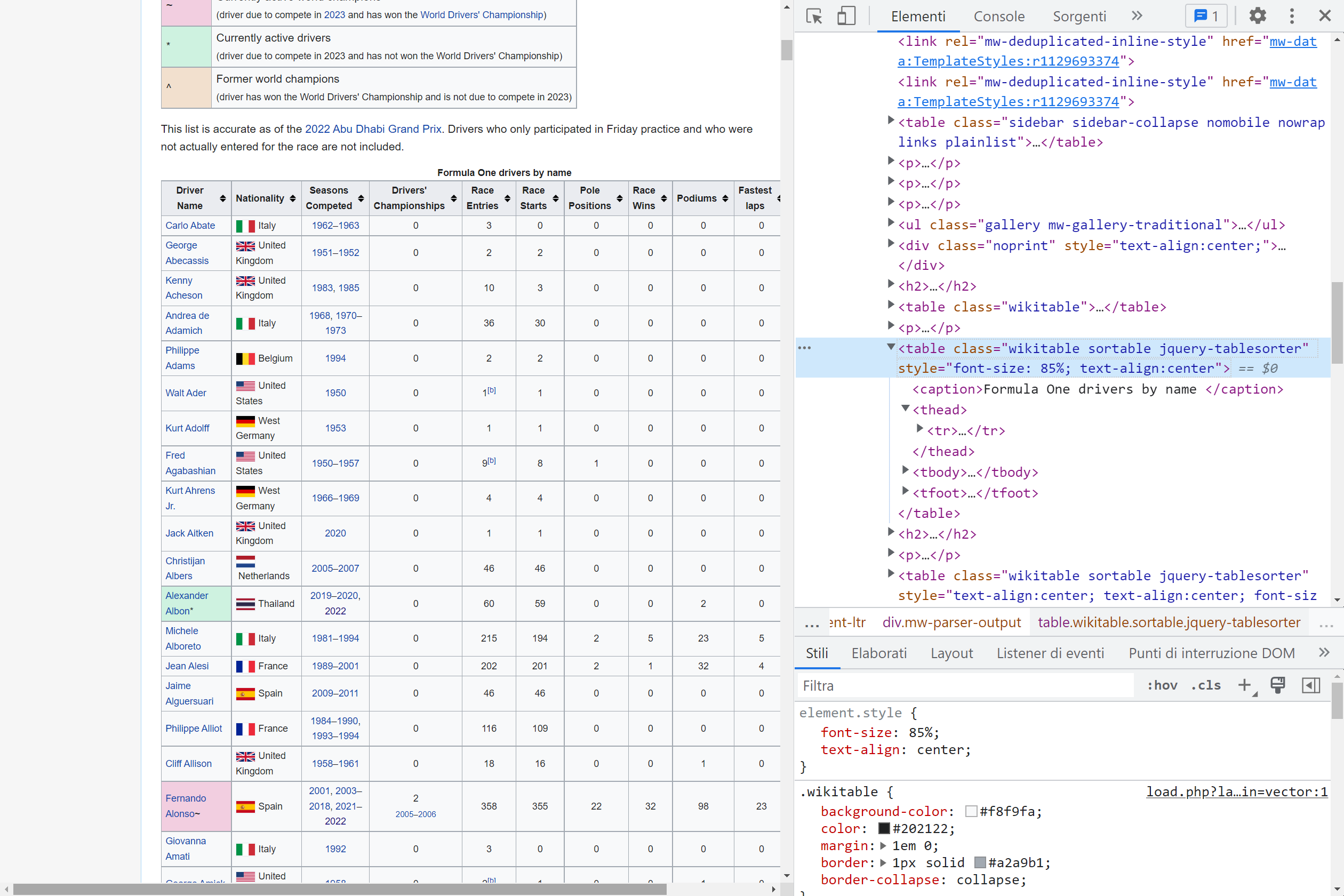
Therefore we run the following lines of code:
drivers_F1 <- html_element(page, "table.sortable") %>%
  html_table()
In the chunk of code above, the html_table function is used to render the HTML code into tables.
To inspect it, we display the first and last observations, and the structure of the dataset:
head(drivers_F1) # first 6 rows## # A tibble: 6 × 11
## `Driver name` Nationality `Seasons competed` `Drivers' Championships`
## <chr> <chr> <chr> <chr>
## 1 Carlo Abate Italy 1962–1963 0
## 2 George Abecassis United Kingdom 1951–1952 0
## 3 Kenny Acheson United Kingdom 1983, 1985 0
## 4 Andrea de Adamich Italy 1968, 1970–1973 0
## 5 Philippe Adams Belgium 1994 0
## 6 Walt Ader United States 1950 0
## # ℹ 7 more variables: `Race entries` <chr>, `Race starts` <chr>,
## # `Pole positions` <chr>, `Race wins` <chr>, Podiums <chr>,
## # `Fastest laps` <chr>, `Points[a]` <chr>tail(drivers_F1) # last 6 rows## # A tibble: 6 × 11
## `Driver name` Nationality `Seasons competed` `Drivers' Championships`
## <chr> <chr> <chr> <chr>
## 1 Emilio Zapico Spain 1976 0
## 2 Zhou Guanyu China 2022–2024 0
## 3 Ricardo Zonta Brazil 1999–2001, 2004–2005 0
## 4 Renzo Zorzi Italy 1975–1977 0
## 5 Ricardo Zunino Argentina 1979–1981 0
## 6 Driver name Nationality Seasons competed Drivers' Championships
## # ℹ 7 more variables: `Race entries` <chr>, `Race starts` <chr>,
## # `Pole positions` <chr>, `Race wins` <chr>, Podiums <chr>,
## # `Fastest laps` <chr>, `Points[a]` <chr>str(drivers_F1) # structure of the dataset## tibble [878 × 11] (S3: tbl_df/tbl/data.frame)
## $ Driver name : chr [1:878] "Carlo Abate" "George Abecassis" "Kenny Acheson" "Andrea de Adamich" ...
## $ Nationality : chr [1:878] "Italy" "United Kingdom" "United Kingdom" "Italy" ...
## $ Seasons competed : chr [1:878] "1962–1963" "1951–1952" "1983, 1985" "1968, 1970–1973" ...
## $ Drivers' Championships: chr [1:878] "0" "0" "0" "0" ...
## $ Race entries : chr [1:878] "3" "2" "10" "36" ...
## $ Race starts : chr [1:878] "0" "2" "3" "30" ...
## $ Pole positions : chr [1:878] "0" "0" "0" "0" ...
## $ Race wins : chr [1:878] "0" "0" "0" "0" ...
## $ Podiums : chr [1:878] "0" "0" "0" "0" ...
## $ Fastest laps : chr [1:878] "0" "0" "0" "0" ...
## $ Points[a] : chr [1:878] "0" "0" "0" "6" ...Now that we have a tibble (a sort of dataframe used in the tidyverse universe), we just need to select the variables of interest and eliminate the last row that contains the name of the variables:
drivers_F1 <- drivers_F1[c(1:4, 7:9)] # select variables

drivers_F1 <- drivers_F1[-nrow(drivers_F1), ] # remove last row
At this point we may want to clean our data. For example, we notice that Drivers' Championships has a small formatting issue: it returns not only the number of championships the driver won, but also the years of the victories. To extract only the number of victories (without the years) we use the substr() function:
drivers_F1$`Drivers' Championships` <- substr(drivers_F1$`Drivers' Championships`,
  start = 1, stop = 1
)
With this code, we actually extract only the first character since we start at 1 and stop at 1. At the moment, the maximum number of championships won by a driver is 7 (Lewis Hamilton & Michael Schumacher), so it is fine to extract only the first digit.
Et voila! With only a few lines of code, we scraped a table and we are now ready to perform our analysis.
If you want to save the dataset, you can always do so:
write.csv(drivers_F1, "F1_drivers.csv", row.names = FALSE)Analysis on the database
To convince you that this is a real database, we will now answer some simple questions.
First of all, we load the tidyverse package:
library(tidyverse)- Which country has the largest number of wins?
drivers_F1 %>%
  group_by(Nationality) %>%
  summarise(championship_country = sum(as.double(`Drivers' Championships`))) %>%
  arrange(desc(championship_country))
## # A tibble: 48 × 2
## Nationality championship_country
## <chr> <dbl>
## 1 United Kingdom 21
## 2 Germany 12
## 3 Brazil 8
## 4 Argentina 5
## 5 Australia 4
## 6 Austria 4
## 7 Finland 4
## 8 France 4
## 9 Netherlands 4
## 10 Italy 3
## # ℹ 38 more rows- Who has the most Championships?
drivers_F1 %>%
  group_by(`Driver name`) %>%
  summarise(championship_pilot = sum(as.double(`Drivers' Championships`))) %>%
  arrange(desc(championship_pilot))
## # A tibble: 877 × 2
## `Driver name` championship_pilot
## <chr> <dbl>
## 1 Lewis Hamilton~ 7
## 2 Michael Schumacher^ 7
## 3 Juan Manuel Fangio^ 5
## 4 Alain Prost^ 4
## 5 Max Verstappen~ 4
## 6 Sebastian Vettel^ 4
## 7 Ayrton Senna^ 3
## 8 Jack Brabham^ 3
## 9 Jackie Stewart^ 3
## 10 Nelson Piquet^ 3
## # ℹ 867 more rowsSorry Michael, it looks like Lewis dethroned you.
- Is there a relation between the number of Championships won and the number of race pole positions?
drivers_F1 %>%
  filter(`Pole positions` > 1) %>%
  ggplot(aes(x = as.double(`Pole positions`), y = as.double(`Drivers' Championships`))) +
  geom_point(position = "jitter") +
  labs(y = "Championships won", x = "Pole positions") +
  theme_minimal()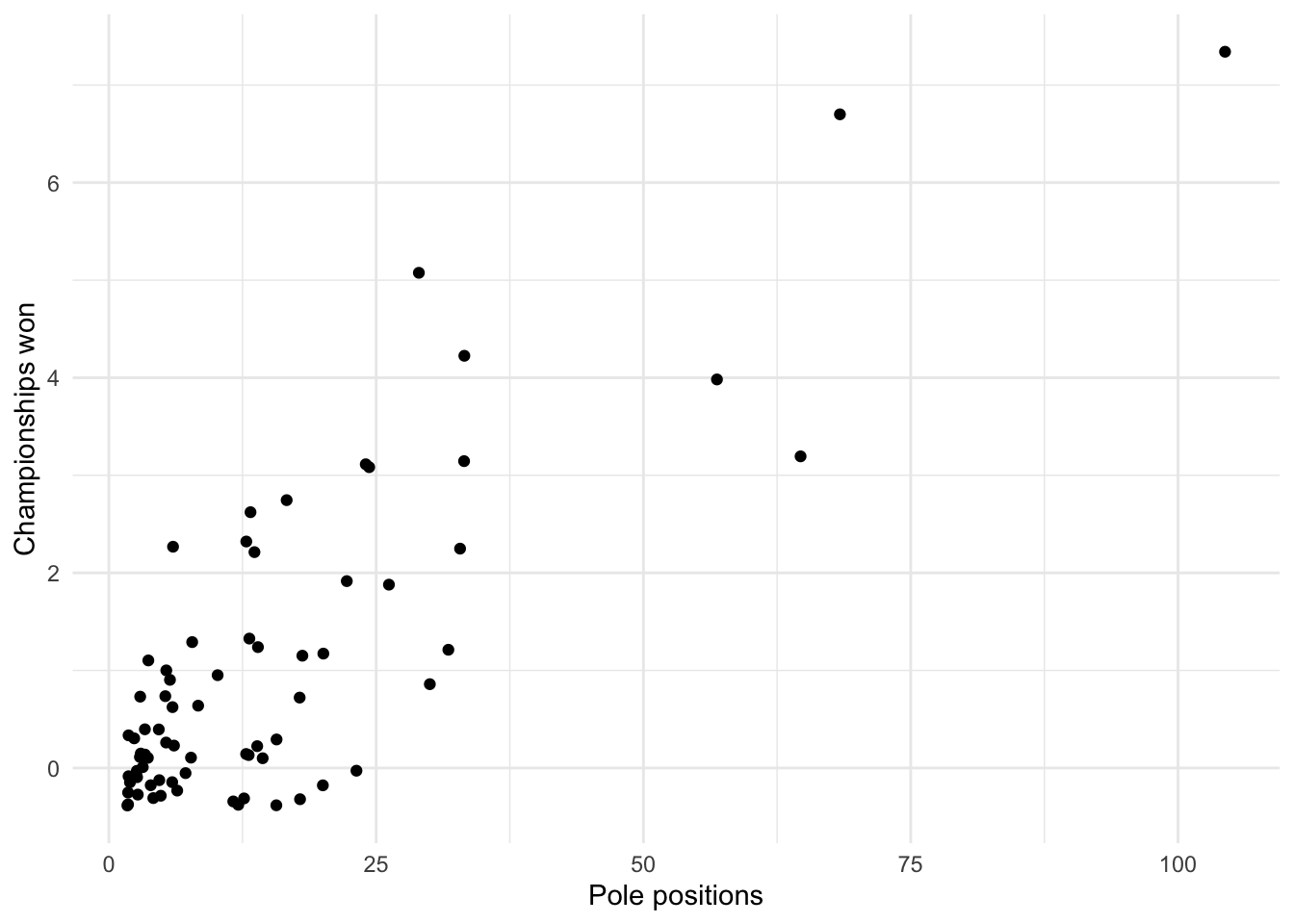
As expected, there seems to be a positive relationship between the number of pole positions and the number of Championships won. To quantify this relationship, we could build a linear model but this is beyond the scope of the article.
To go further
As you have seen, rvest is a powerful tool. The goal of the article is to show just the tip of the iceberg regarding web scraping in R.
There are many resources online that you can read if you want to know more:
- Web scraping: Basics by Paul Bauer
- rvest CRAN documentation
- xml2 CRAN documentation
- httr CRAN documentation
- rvest CRAN vignette
- httr CRAN vignette
- Beautiful Soup documentation
- RoboBrowser documentation
- HTML documentation
- CSS documentation
Conclusion
Thanks for reading.
I hope this article helped you to learn about web scraping in R, and gave you the incentive to use it for your projects. If you are interested in seeing another example, see how to scrape Yahoo search engine results with R.
As always, if you have a question or a suggestion related to the topic covered in this article, please add it as a comment so other readers can benefit from the discussion.
Liked this post?
- Get updates every time a new article is published (no spam and unsubscribe anytime)
- Support the blog
- Share on:


