What is R and RStudio?

How to install R and RStudio?

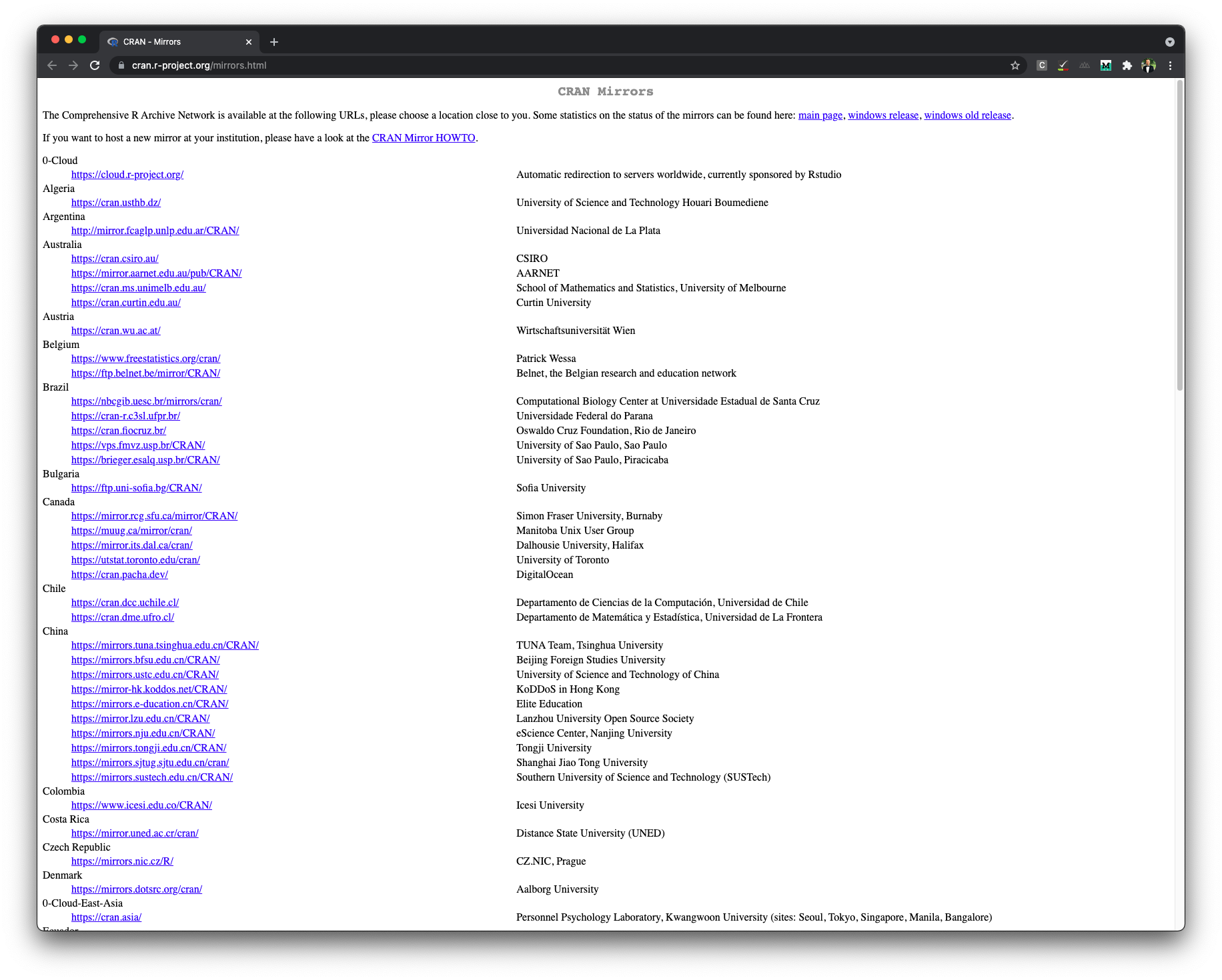
You can download R at https://cran.r-project.org/mirrors.html. Select the CRAN mirror site closest to your country. If there are more than one links for your country, simply select one:

Select the CRAN mirror site closest to your country

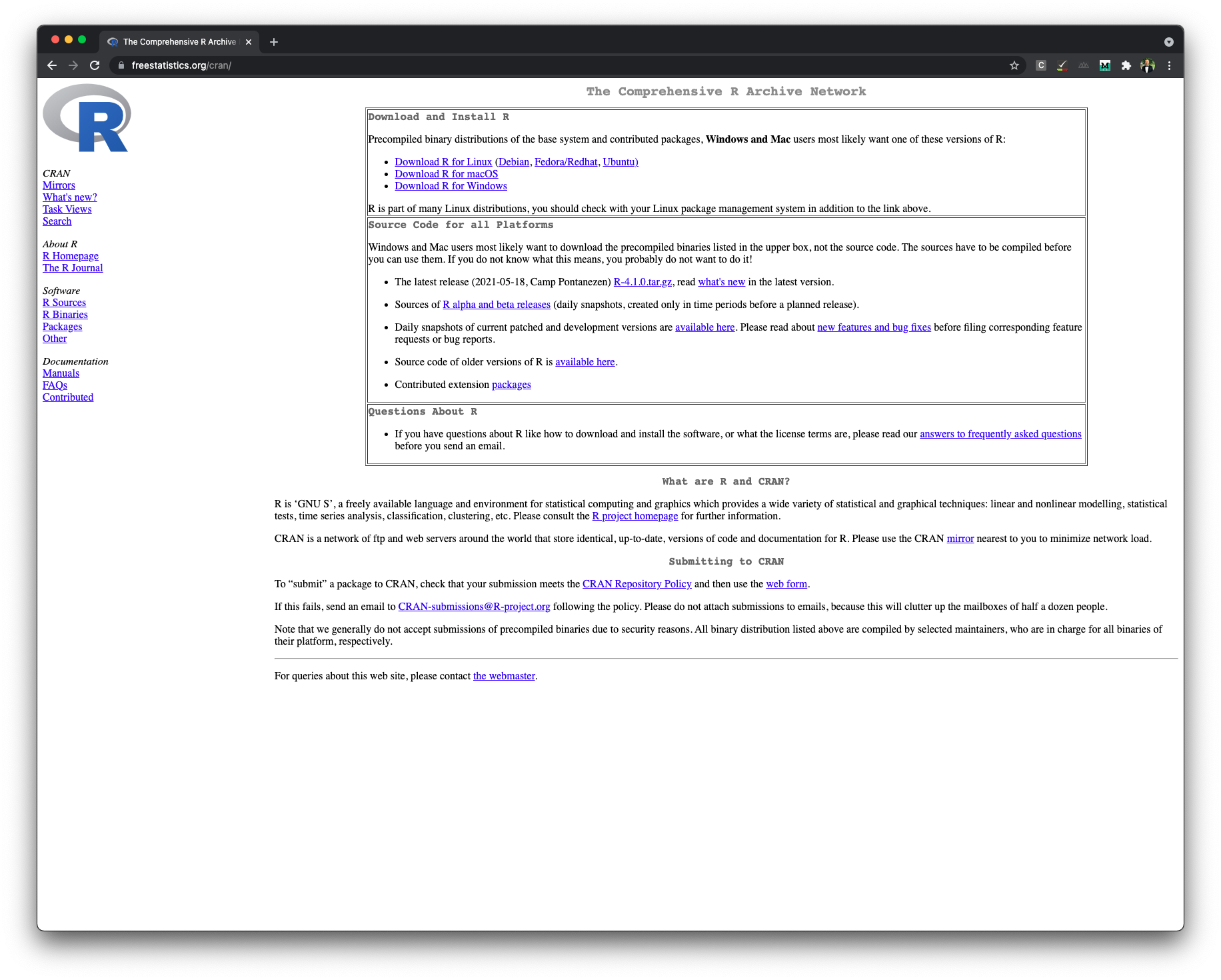
Then in the box labeled “Download and Install R” (located at the top), click on the link corresponding to your operating system (Windows, Mac or Linux):

Click on the link corresponding to your operating system

Now that R is installed on your computer, you can download RStudio. You can download the free version of RStudio (which is totally enough for most users, including me!) on their website.

The main components of RStudio

Now that both programs are installed on your computer, let’s dive into the main components of RStudio.

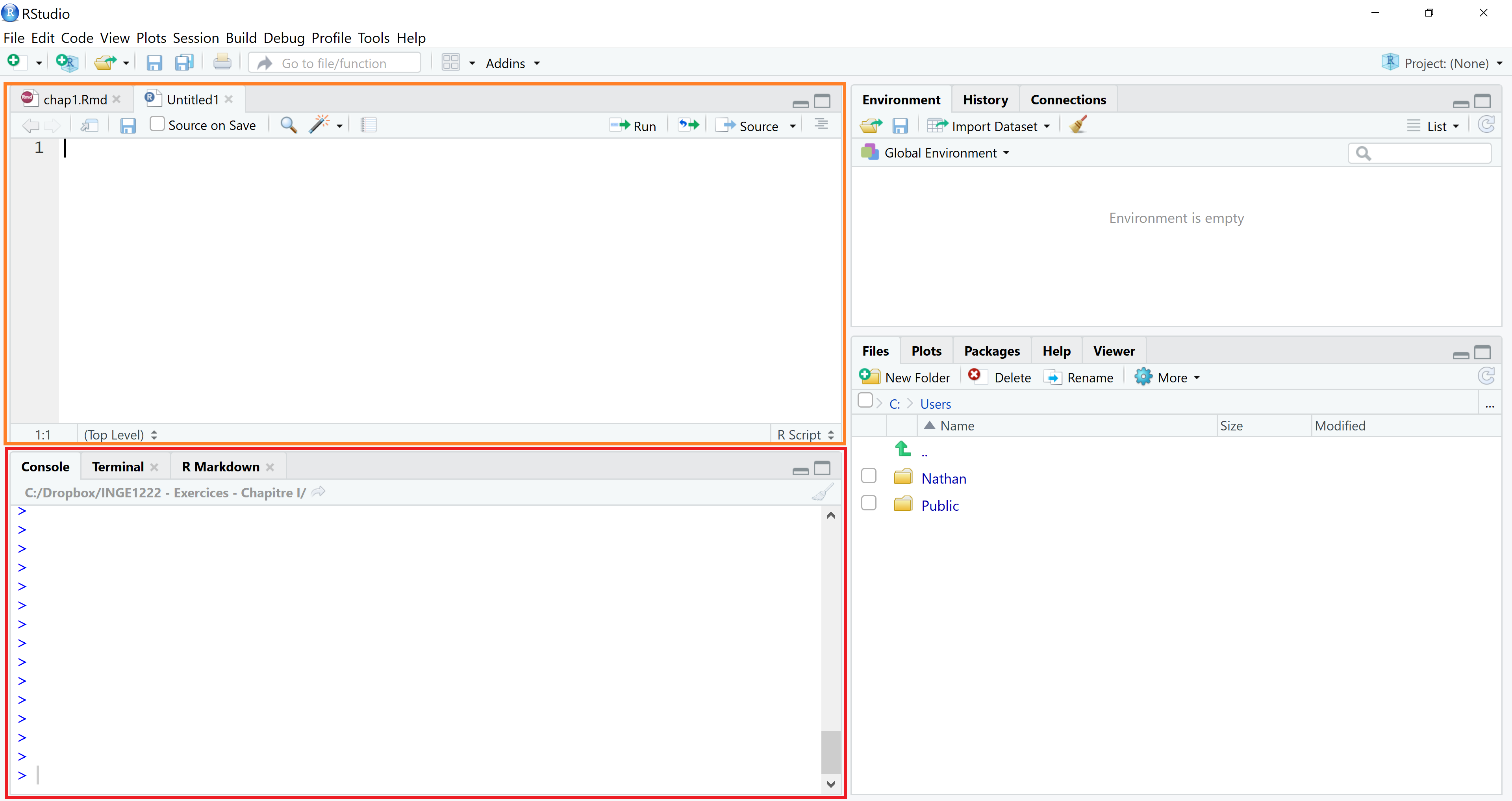
By default, the RStudio window has three panes:

1. The console (red pane)
2. The environment (green pane)
3. Files, plots, help, etc. (blue pane)

RStudio window

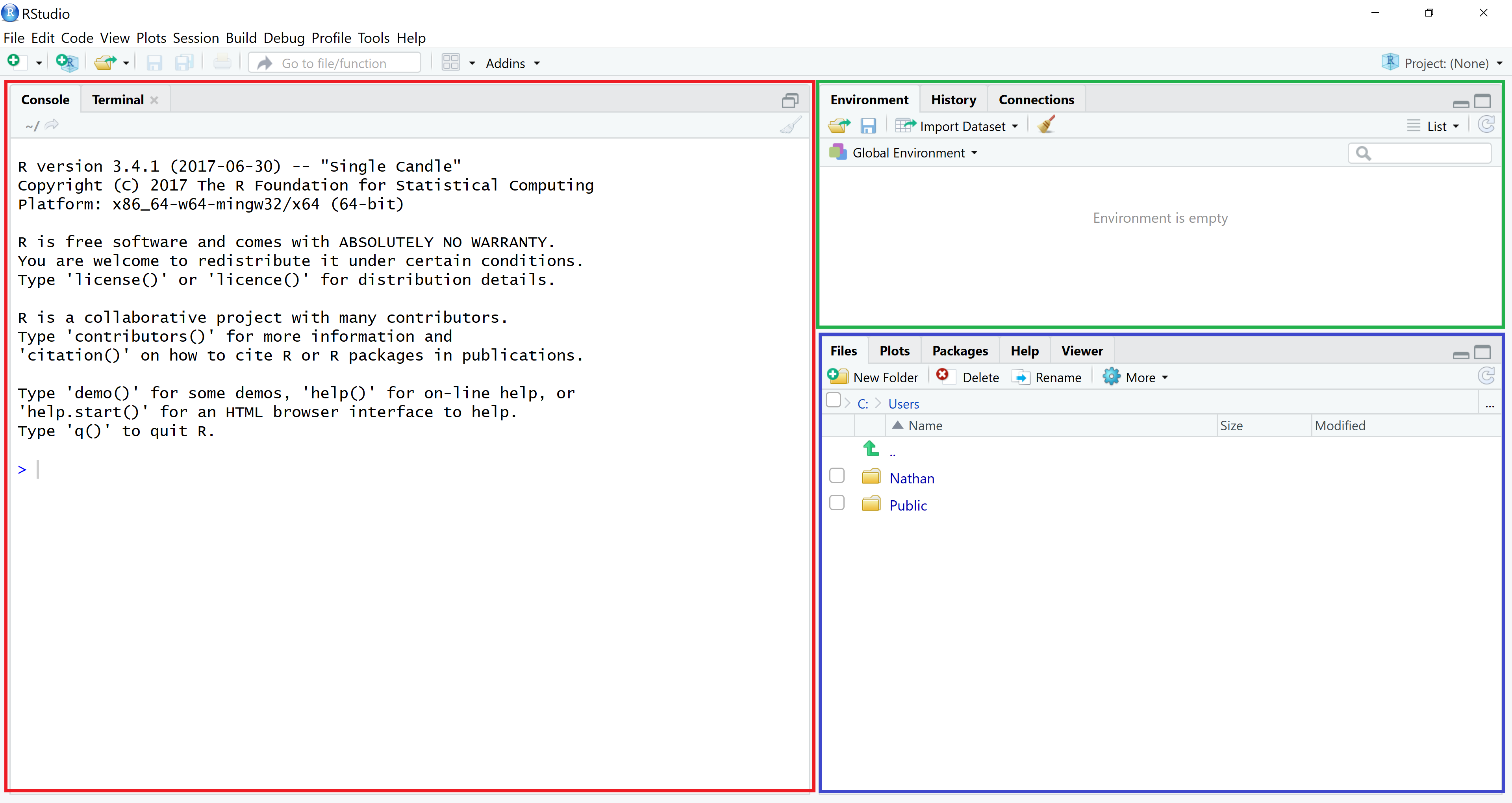
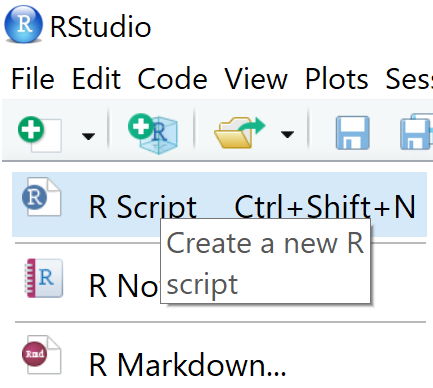
The console (red pane) is where you can execute your code (more information on the red and blue panes later). By default, the text editor does not open automatically. To open it, click on File > New File > R Script or click on the button representing a white sheet marked with a small green cross in the upper left corner, then on R Script:

New R script in RStudio

A new pane (in orange below), also known as the text editor, opens in which you will be able to write your code. The code will be executed and the results displayed in the console (red pane).

Write and execute your code in RStudio

Note that you can also write code in the console (red pane). However, I strongly recommend writing your code in the text editor (orange pane) because you can save the code written in the text editor (and thus execute it again later), while you cannot save the code written in the console.

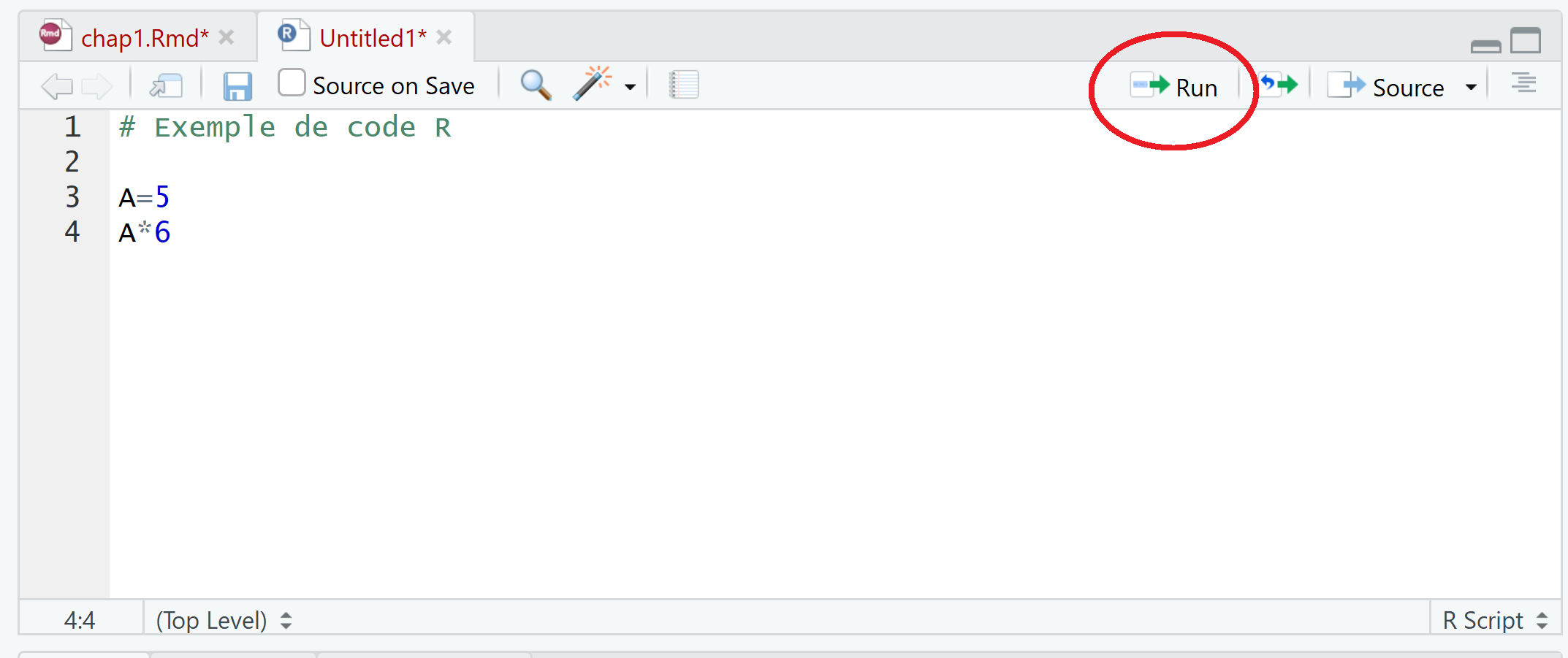
To execute code written in the text editor (orange pane), you have two options:

• Type your code and then press the “Run” button (see below) or use the keyboard shortcut CTRL + Enter (cmd + Enter on Mac). Only the chunk of code where your cursor is located will then be executed.
• Type your code and select in the text editor the part you want to execute and then press the “Run” button or use the keyboard shortcut CTRL + Enter (cmd + Enter on Mac). All the selected code will be executed

Run code in RStudio

For example, try typing 1+1 in the text editor and execute it by clicking on “Run” (or CTRL/cmd + Enter). You should see the result 2 in the console, as shown in the screenshot below:

Example of code executed in RStudio

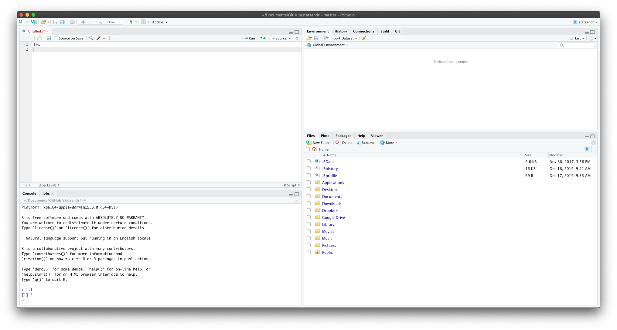
The text editor and the console are the panes you will use most often. The two other panes (the blue and green panes introduced earlier) will however still be very useful when using RStudio.

The environment (green pane) displays all values stored by RStudio. For example, if you type and execute the code a = 1, RStudio will store the value 1 for a, as shown in the screenshot below:

Environment pane in RStudio

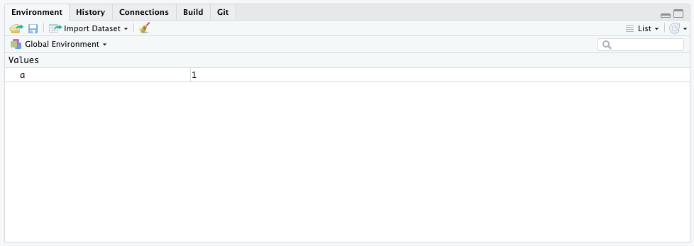
This means that you can now perform any computations with a, such that if you execute a + 1, RStudio will render 2 in the console. In this pane you can also see a tab with a history of the code executed and a button to import a dataset (more on importing a dataset in RStudio).

The last pane (blue) is where you will find everything else such as your files, the plots, the packages, the help documentation, etc. I discuss about the Files tab in more detail here so let’s discuss about the other tabs:

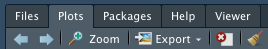
• Plot: where you will see the rendered plots. For instance, run plot(1:10) and you should see it in this tab. If you plotted more than one plots, you can navigate between them by clicking on the arrows. You can open the plot in a new window by clicking on Zoom and export your plot by clicking on Export. Those buttons are located just under the Plot tab (see figure below)
• Packages: where you see all your installed packages. Only fundamental functionalities come with R. Everything else must be installed from packages. Remind that R is open source; everyone can write code and publish it as a package. You are then able to use this package (and all functions built inside this package) for free. 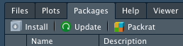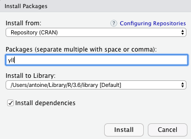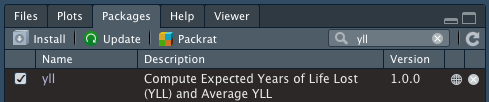Some packages are installed by default, all others must be installed by running install.packages("name of the package") (do not forget "" around the name of the package!). Once the package is installed, you must load the package and only after it has been loaded you can use all the functions it contains. To load a package, run library(name of the package) (this time "" around the name of the package are optional, but can still be used if you wish). You also have the possibility to install and load packages via the buttons under the Packages tab. For this, click on the button Install under Packages, type the name of the package you want to install and then click on Install. You will see that the code appears in the console. To load the package, find the package you want to load in the Packages window (you can use the search box), then click on the checkbox next to the name of the package. Again, the code is run in the console. See the figures below if needed. Note that you will need to install packages only once,¹ but load packages each time you open RStudio. Furthermore, note that an internet connection is required to install a package, while it is not required to load a package
• Help: documentation about all functions written for R. To access the help of a function, run help("name of the function") or simply ?name of the function. For example, to see the help about the mean function, run ?mean. You can also press F1 while having your cursor on a function

Plot buttons in RStudio

Step 1: click on the Install button

Step 2: type the name of the package and click on Install

Step 3: load your package by clicking on the box next to the package’s name

Examples of code

Now that you have installed R and RStudio and you know its main components, below are some examples of basic code.

More advanced code and analyses are presented in other articles about R, and in particular in this article about data manipulation in R.

5 * 5

## [1] 25

1 / sqrt(50 * pi) * exp(-(10 - 11)^2 / 50)

## [1] 0.07820854

# A comment
# Another comment
1 + 1

## [1] 2

A <- 5
B <- 6

(A <- 5)

## [1] 5

A <- 5
A

## [1] 5

A <- c(1 / 2, -1, 0)
A

## [1]  0.5 -1.0  0.0

my_mat <- matrix(c(-1, 2, 0, 3), ncol = 2, nrow = 2)
my_mat

##      [,1] [,2]
## [1,]   -1    0
## [2,]    2    3

my_mat2 <- matrix(c(-1, 2, 0, 3), nrow = 2, ncol = 2)
my_mat2

##      [,1] [,2]
## [1,]   -1    0
## [2,]    2    3

my_mat == my_mat2 # is my_mat equal to my_mat2?

##      [,1] [,2]
## [1,] TRUE TRUE
## [2,] TRUE TRUE

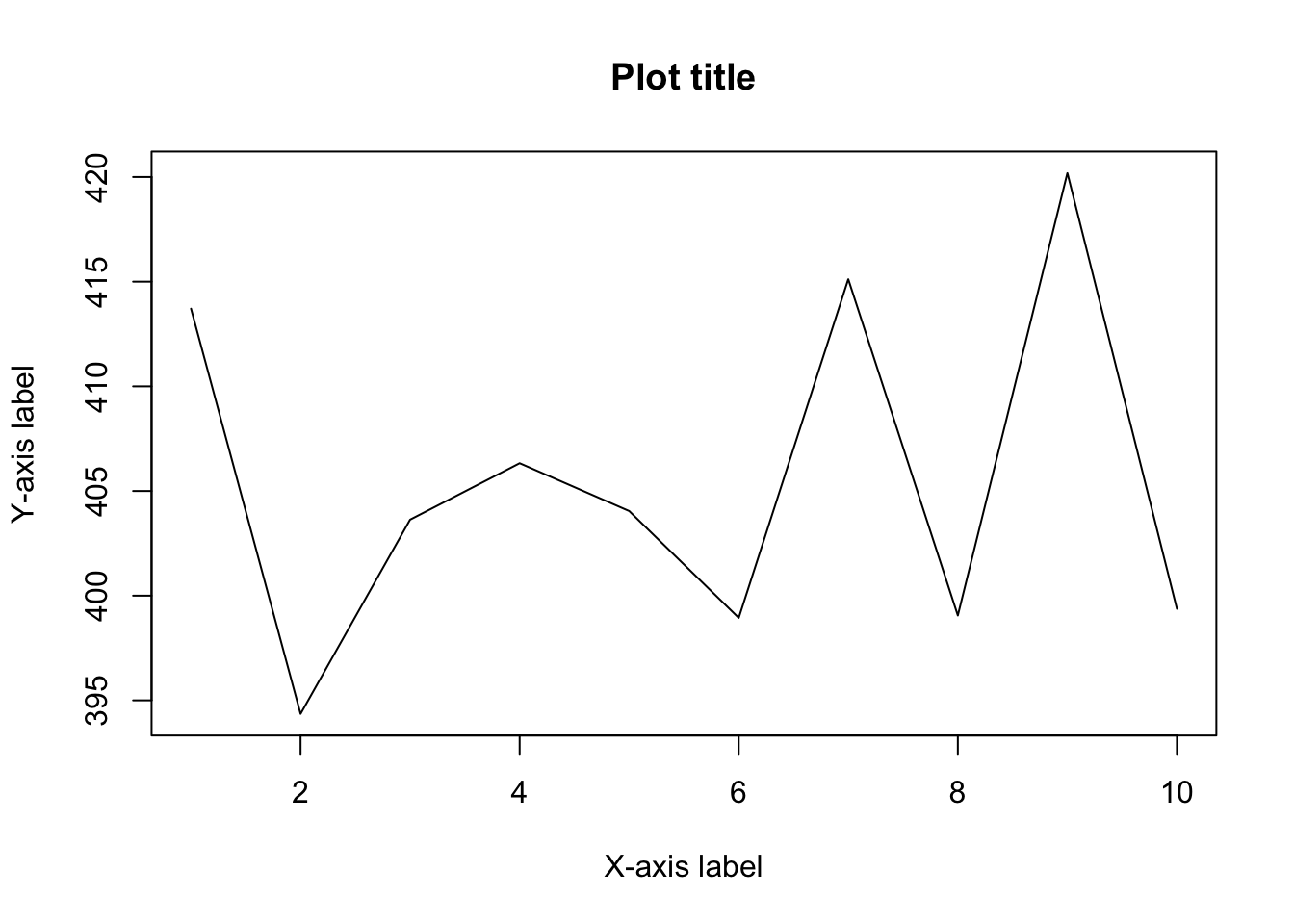
my_vec <- rnorm(10, mean = 400, sd = 10)
# Display only the first 5 values:
head(my_vec, 5)

## [1] 413.7096 394.3530 403.6313 406.3286 404.0427

# Display only the last 5 values:
tail(my_vec, 5)

## [1] 398.9388 415.1152 399.0534 420.1842 399.3729

set.seed(42)
rnorm(3, mean = 10, sd = 2)

## [1] 12.741917  8.870604 10.726257

plot(my_vec,
  type = "l", # "l" stands for line
  main = "Plot title",
  ylab = "Y-axis label",
  xlab = "X-axis label"
)

Conclusion

Thanks for reading.

I hope this article helped you to install R and RStudio.

This is only a very limited introduction to the possibilities of RStudio. If you want to learn more, I recommend that you read other articles related to R, starting with how to import an Excel file or how to manipulate a dataset in R.

As always, if you have a question or a suggestion related to the topic covered in this article, please add it as a comment so other readers can benefit from the discussion.