Repeated measures ANOVA in R

Introduction
In a previous article, we presented the one-way ANOVA, the statistical test used to compare a quantitative variable between three groups or more. One of its assumptions was stated very explicitly in that article: the observations must be independent, both within and between the groups. It was also mentioned that if observations between samples are dependent (for example, if three measurements have been collected on the same individuals, as it is often the case in medical studies when a metric is measured (i) before, (ii) during and (iii) after a treatment), the repeated measures ANOVA should be preferred. The present article is dedicated to that test.
The repeated measures ANOVA compares the means of a quantitative variable measured several times on the same subjects, that is, under \(k \geq 3\) related conditions or at \(k \geq 3\) different points in time. The aim is exactly the same as the aim of the one-way ANOVA (testing whether the means are equal across the \(k\) conditions), but the design is different: instead of \(k\) independent groups formed by different subjects, we have a single group of subjects who go through all the conditions. The factor whose levels are the conditions is then called a within-subjects factor, as opposed to the between-subjects factor of the one-way ANOVA.
The relationship between the two tests mirrors the relationship between the two versions of the Student’s t-test:
| Independent samples | Related samples | |
|---|---|---|
| 2 groups | Student’s t-test for independent samples | Student’s t-test for paired samples |
| 3 groups or more | One-way ANOVA | Repeated measures ANOVA |
In other words, the repeated measures ANOVA is to the paired Student’s t-test what the one-way ANOVA is to the Student’s t-test for independent samples: the generalization of the same logic to three groups or more. This is also why the repeated measures ANOVA appears in the list of related methods presented in the article about the two-way ANOVA, next to the mixed ANOVA (used when a between-subjects factor and a within-subjects factor are present at the same time).
Taking the repeated structure of the data into account is not a detail, and it is beneficial for two reasons:
- Analyzing repeated measurements as if they came from independent groups violates the independence assumption of the one-way ANOVA, so the results of that test could simply not be trusted.
- Since each subject serves as its own control, the variability between subjects (the fact that some patients are, in general, more sensitive to pain than others, for instance) is isolated and removed from the error term. The test is therefore usually more powerful than a one-way ANOVA run on the same number of measurements.
The price to pay for this gain is an additional assumption, called sphericity, which does not exist in the independent-groups case and which is discussed in detail in this article.
In the remaining of the post, we present the data, the aim, the hypotheses and the assumptions of the test, and we finally show how to perform it in R, how to complement it with post-hoc tests and how to interpret the results.
Data
Datasets with a genuinely repeated structure are not so common among the datasets shipped with R, so we simulate our own data. This has the additional advantage that we know exactly how the data have been generated.
Suppose that a treatment against chronic pain is administered to 30 randomly selected patients, and that the intensity of the pain is measured on each patient on a scale from 0 (no pain at all) to 100 (unbearable pain) at three different moments:
- before the treatment,
- during the treatment, and
- one month after the end of the treatment, in order to see whether the benefit of the treatment persists over time.
# number of patients
n <- 30

# each patient has its own baseline level of pain
patient_effect <- rnorm(n, mean = 0, sd = 8)

# pain score at the 3 moments
before <- 70 + patient_effect + rnorm(n, mean = 0, sd = 6)
during <- 63 + patient_effect + rnorm(n, mean = 0, sd = 6)
after <- 61.5 + patient_effect + rnorm(n, mean = 0, sd = 6)

# dataset in the long format
dat <- data.frame(
  patient = factor(rep(1:n, times = 3)),
  time = factor(rep(c("before", "during", "after"), each = n),
    levels = c("before", "during", "after")
  ),
  pain = round(c(before, during, after), 1)
)

str(dat)
## 'data.frame': 90 obs. of 3 variables:
## $ patient: Factor w/ 30 levels "1","2","3","4",..: 1 2 3 4 5 6 7 8 9 10 ...
## $ time : Factor w/ 3 levels "before","during",..: 1 1 1 1 1 1 1 1 1 1 ...
## $ pain : num 83.7 69.7 79.1 71.4 76.3 58.8 77.4 64.1 71.7 69.7 ...head(dat)## patient time pain
## 1 1 before 83.7
## 2 2 before 69.7
## 3 3 before 79.1
## 4 4 before 71.4
## 5 5 before 76.3
## 6 6 before 58.8(Note that a seed has been set in the background with set.seed(42), so the simulated data and all the results presented below are reproducible.)
Two points are worth being highlighted in the code above:
- The term
patient_effectis added to the three measurements of the same patient. This is what creates the dependency between the three scores of a given patient: a patient with a high baseline level of pain tends to have a high score at all three moments. - The data are stored in the long format, with one row per patient and per measurement, and three variables: the identifier of the subject (
patient), the within-subjects factor (time) and the quantitative variable of interest (pain). This is the format expected by the functions used in the rest of the article. If your data are in the wide format (one row per subject and one column per condition), they can be reshaped with thepivot_longer()function of the{tidyr}package.
As always, it is a good practice to start with some descriptive statistics, here the mean and the standard deviation of the pain score at each of the three moments:
# install.packages("dplyr")
library(dplyr)

dat %>%
  group_by(time) %>%
  summarise(
    n = n(),
    mean = mean(pain),
    sd = sd(pain)
  )
## # A tibble: 3 × 4
## time n mean sd
## <fct> <int> <dbl> <dbl>
## 1 before 30 69.8 10.7
## 2 during 30 64.7 10.5
## 3 after 30 61.9 11.5The boxplots below give a first visual comparison of the three moments:
# install.packages("ggplot2")
library(ggplot2)

ggplot(dat) +
  aes(x = time, y = pain) +
  geom_boxplot() +
  labs(
    x = "Moment of the measurement",
    y = "Pain score"
  )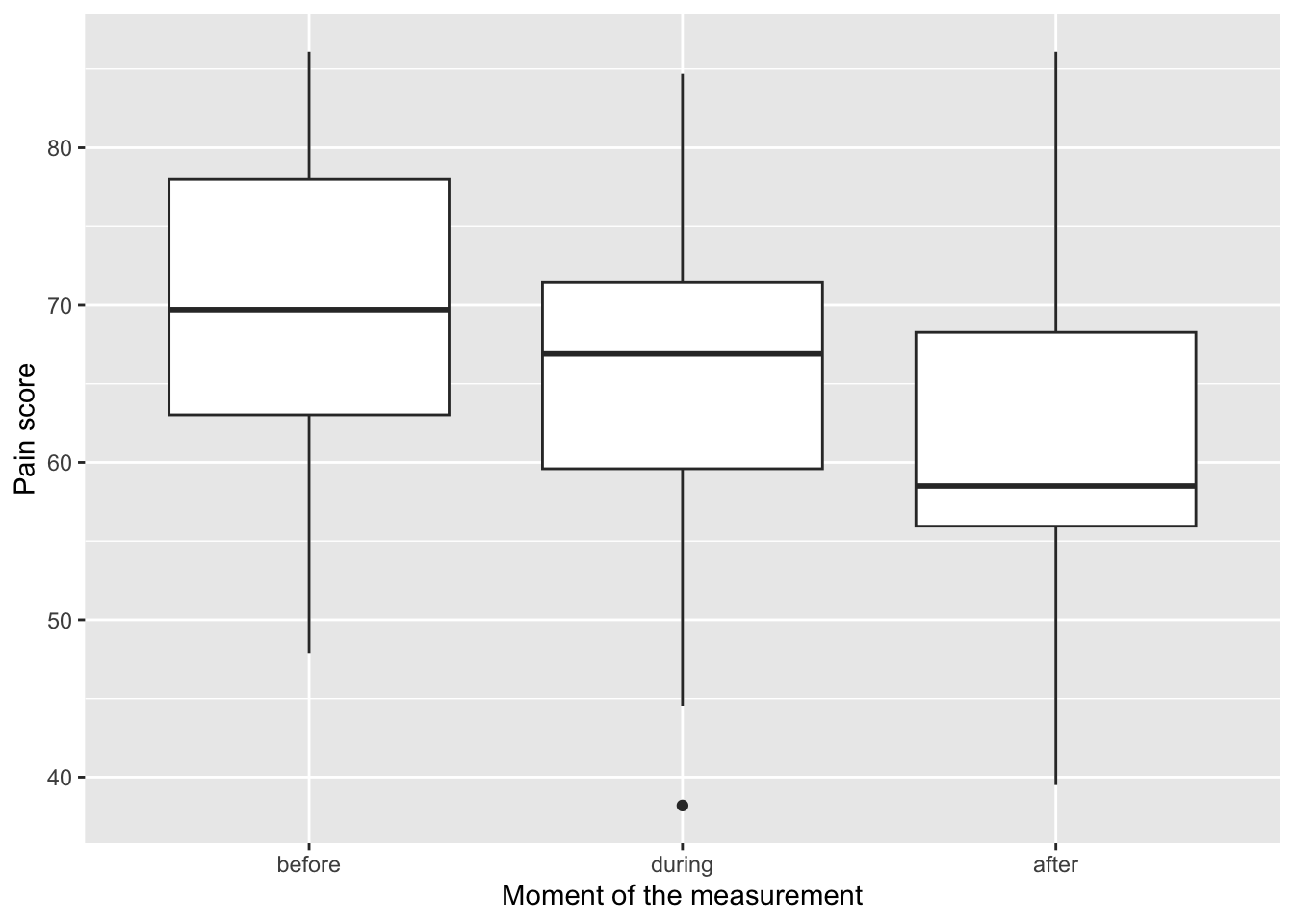
Boxplots are, however, not entirely satisfactory here because they completely hide the repeated structure of the data. A plot which is much better suited to repeated measurements is the so-called spaghetti plot, where the successive scores of each patient are joined by a line (the thick blue line represents the mean at each moment):
ggplot(dat) +
  aes(x = time, y = pain, group = patient) +
  geom_line(alpha = 0.3) +
  geom_point(alpha = 0.3) +
  stat_summary(aes(group = 1),
    fun = mean, geom = "line",
    linewidth = 1.2, color = "steelblue"
  ) +
  stat_summary(aes(group = 1),
    fun = mean, geom = "point",
    size = 3, color = "steelblue"
  ) +
  labs(
    x = "Moment of the measurement",
    y = "Pain score"
  )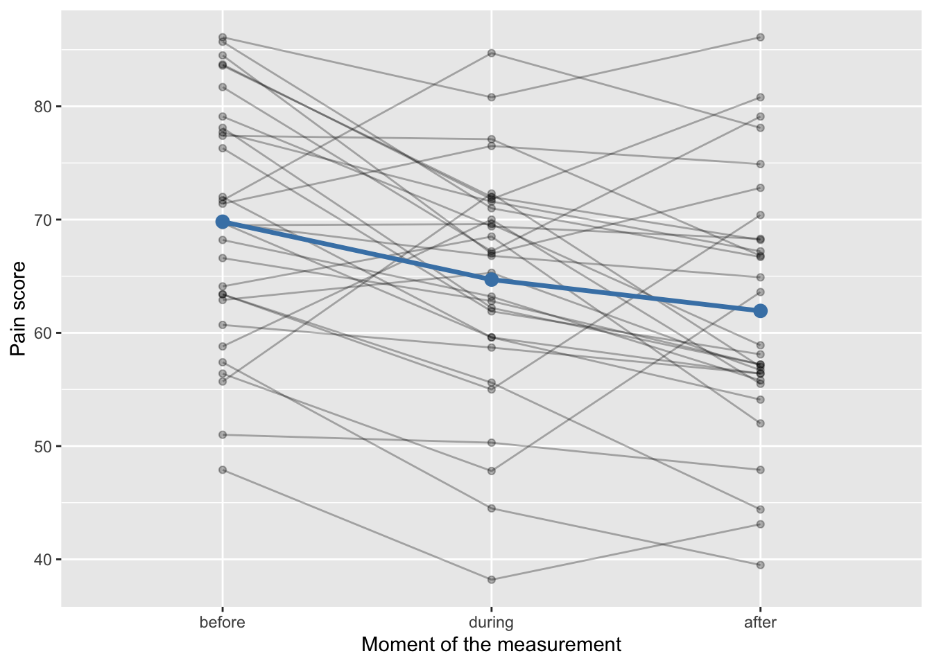
In our sample, the mean pain score decreased from 69.8 before the treatment to 64.7 during the treatment, and to 61.9 one month after it. The spaghetti plot also shows that most (but not all) patients follow this downward trend, and that the general level of pain varies a lot from one patient to another, which is precisely the between-subjects variability that the repeated measures ANOVA is able to set aside.
The question is now whether these differences are large enough to be generalized to the population, or whether they could be explained by sampling fluctuations alone. This is where the repeated measures ANOVA comes into play.
Aim and hypotheses
As explained in the introduction, the repeated measures ANOVA is used to compare the means of a quantitative variable measured on the same subjects under \(k \geq 3\) related conditions or at \(k \geq 3\) points in time.
The null and alternative hypotheses of the test are:
- \(H_0\): the population means are equal in all \(k\) related conditions, that is, \(\mu_1 = \mu_2 = \dots = \mu_k\)
- \(H_1\): at least one condition is different from the others in terms of mean
Be careful that, exactly as for the one-way ANOVA or the Kruskal-Wallis test, the alternative hypothesis is not that all means are different from each other. The opposite of “all means are equal” (\(H_0\)) is “at least one mean is different from the others” (\(H_1\)). So if the null hypothesis is rejected, we only know that at least one moment differs from the others, and post-hoc tests (covered later in this article) must be performed in order to know which ones actually differ.
In the context of our example, the repeated measures ANOVA helps us to answer the following question: “Is the mean pain score the same before, during and after the treatment?”. With the notations of our dataset, the hypotheses become:
- \(H_0\): \(\mu_{before} = \mu_{during} = \mu_{after}\)
- \(H_1\): at least one of the three moments differs from the others in terms of mean pain score
Note that, as its name suggests, the test still works by comparing variances: the variability observed between the conditions is compared to the residual variability, but this time after having removed the variability due to the subjects themselves. This is the reason why the error term of a repeated measures ANOVA is smaller than the error term of a one-way ANOVA computed on the same data, and why the test is generally more powerful.
Assumptions
As for many statistical tests, some assumptions must be met for the results to be valid.
Variable type and design
The repeated measures ANOVA requires one quantitative continuous dependent variable, measured on the same subjects under \(k \geq 3\) levels of a qualitative within-subjects factor (the conditions or the points in time). Ideally, all subjects are measured under all conditions, since subjects with a missing measurement are simply dropped from the analysis.
In our example, the dependent variable is the pain score (quantitative continuous) and the within-subjects factor is the moment of the measurement, with 3 levels (before, during and after the treatment), all measured on the same 30 patients. This assumption is thus met.
Note that if only 2 related measurements were available, the Student’s t-test for paired samples would be used instead, and if the \(k\) samples were independent, the one-way ANOVA would be the appropriate test.
Independence between subjects
Independence is required between subjects, but not within them. This point is often a source of confusion, so it is worth insisting on it: the \(k\) measurements of a given patient are of course dependent (this is the whole point of the design, and it is exactly what the test accounts for), but the measurements of one patient must not influence the measurements of another patient.
As for many tests, this assumption is verified based on the design of the experiment and on the good control of the experimental conditions rather than via a formal test. Here, patients have been selected at random and treated individually, so we consider this assumption to be met.
Normality
For small samples, the residuals of the model (equivalently, the differences between the conditions) should follow approximately a normal distribution. As for the one-way ANOVA, this requirement becomes much less critical when the number of subjects is large, thanks to the central limit theorem: with a large enough sample, the sampling distribution of the means is well approximated by a normal distribution even if the data themselves are not normally distributed.
With only 30 patients, we are in a borderline situation, so it is safer to check normality. The residuals of interest are those obtained after having removed both the effect of the moment and the effect of the patient, so they can be computed from a linear model including these two factors:
# residuals of the model, taking the patient effect into account
res_lm <- lm(pain ~ time + patient, data = dat)
Normality can then be assessed visually via a histogram and a QQ-plot:
par(mfrow = c(1, 2)) # combine plots

hist(residuals(res_lm),
  main = "Histogram of the residuals",
  xlab = "Residuals"
)

# install.packages("car")
library(car)

qqPlot(residuals(res_lm),
  id = FALSE # remove point identification
)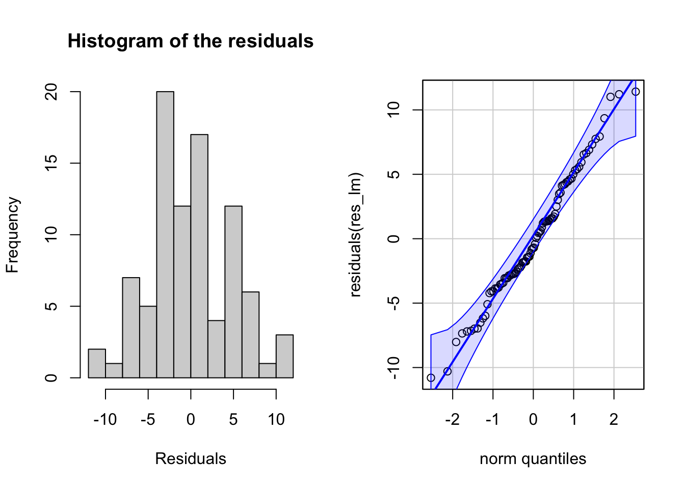
The histogram is roughly symmetric around zero and the points of the QQ-plot are close to the straight line and all inside the confidence bands, so the normality assumption seems reasonable.
If you prefer a formal normality test, the Shapiro-Wilk test can be applied on the same residuals:
shapiro.test(residuals(res_lm))##
## Shapiro-Wilk normality test
##
## data: residuals(res_lm)
## W = 0.98388, p-value = 0.331The \(p\)-value being larger than the usual significance level of 0.05, we do not reject the hypothesis that the residuals follow a normal distribution, which confirms the visual approach.
If, even after a transformation of the data, normality was clearly not satisfied, the nonparametric alternative to the repeated measures ANOVA should be used: the Friedman test, which compares the conditions based on ranks instead of means and which requires neither normality nor sphericity.
Sphericity
Sphericity is the assumption which distinguishes the repeated measures ANOVA from the one-way ANOVA, and it deserves more than one line.
In the independent-groups case, we require homogeneity of the variances: the variance of the dependent variable must be the same in all groups. In the repeated measures case, this condition is replaced by a condition on the differences between the conditions:
Sphericity holds when the variances of the differences between all possible pairs of related conditions are equal in the population.
With \(k\) conditions, there are \(\frac{k(k-1)}{2}\) possible pairs, so with our 3 moments there are 3 differences to consider: during minus before, after minus before, and after minus during. Sphericity requires the three corresponding variances to be (approximately) equal. On our data, these variances can be computed directly:
# install.packages("tidyr")
library(tidyr)

# from the long format to the wide format
dat_wide <- dat %>%
  pivot_wider(names_from = time, values_from = pain)

c(
  "during - before" = var(dat_wide$during - dat_wide$before),
  "after - before" = var(dat_wide$after - dat_wide$before),
  "after - during" = var(dat_wide$after - dat_wide$during)
)
## during - before after - before after - during
## 77.21154 67.05289 69.24033The three variances are of a comparable magnitude, which is a first good sign.
Why does this matter? Because the \(F\) statistic of a repeated measures ANOVA follows a Fisher distribution with the usual degrees of freedom only if sphericity holds. When it does not, the test becomes too liberal: the reported \(p\)-values are too small, and the risk of concluding that the conditions differ when they actually do not is larger than the announced significance level. Note also that sphericity is automatically satisfied when \(k = 2\) (there is then only one difference, so there is nothing to compare), which is another way of seeing why it never shows up in the context of a paired Student’s t-test.
Sphericity is formally tested with Mauchly’s test, whose hypotheses are:
- \(H_0\): sphericity holds (the variances of the differences are equal)
- \(H_1\): sphericity is violated (at least two of these variances are different)
If the \(p\)-value of Mauchly’s test is larger than the significance level, we do not reject sphericity and the usual (uncorrected) results of the ANOVA can be interpreted. If it is smaller, sphericity is rejected and a correction must be applied.
The two most common corrections are the Greenhouse-Geisser and the Huynh-Feldt corrections. Both work in the same way: they estimate a quantity \(\varepsilon\) which measures how far the data are from sphericity, and they multiply the degrees of freedom of the \(F\) test by this \(\varepsilon\). This estimate lies between \(\frac{1}{k-1}\) and 1, the value 1 corresponding to perfect sphericity. Since the degrees of freedom are reduced, the corrected test is more conservative and the corrected \(p\)-value is larger than the uncorrected one. The \(F\) statistic itself is unchanged, only the reference distribution is adjusted. The Greenhouse-Geisser correction tends to underestimate \(\varepsilon\) (so it is the more conservative of the two), while the Huynh-Feldt correction is less conservative and can even return a value above 1, in which case it is set back to 1. A common rule of thumb is to prefer the Greenhouse-Geisser correction when the estimated \(\varepsilon\) is below 0.75, and the Huynh-Feldt correction when it is above 0.75 (Girden 1992).
Two practical remarks:
- Mauchly’s test is known to be sensitive to the sample size (it lacks power with few subjects and detects negligible departures with many) and to deviations from normality. For this reason, many authors recommend reporting the corrected results by default, whatever the conclusion of Mauchly’s test.
- If sphericity is severely violated, alternatives to the corrections exist: a multivariate approach (MANOVA), a linear mixed model, or the nonparametric Friedman test. The MANOVA approach is attractive here because it works directly with the covariance structure of the difference variables and makes no sphericity assumption at all, so it sidesteps the problem entirely rather than correcting for it.
Fortunately, we do not need to compute any of this by hand: as shown in the next section, the function used to perform the test in R reports Mauchly’s test and both corrections along with the ANOVA table.
Outliers
Finally, there should be no significant outliers in any of the conditions, since the test is based on means and means are sensitive to extreme values. The boxplots drawn in the section about the data show one point outside the whiskers for the measurement taken during the treatment, but it is not an extreme value, so we consider that this assumption is met.
Repeated measures ANOVA in R
With the {rstatix} package
Several functions can be used to perform a repeated measures ANOVA in R. The most convenient one is anova_test() from the {rstatix} package, because it reports Mauchly’s test for sphericity and the two sphericity corrections together with the ANOVA table.
The function expects the data in the long format, the name of the dependent variable (dv), the name of the column identifying the subjects (wid) and the name of the within-subjects factor (within):
# install.packages("rstatix")
library(rstatix)

res_aov <- anova_test(
  data = dat,
  dv = pain,
  wid = patient,
  within = time
)

res_aov
## ANOVA Table (type III tests)
##
## $ANOVA
## Effect DFn DFd F p p<.05 ges
## 1 time 2 58 13.464 1.57e-05 * 0.085
##
## $`Mauchly's Test for Sphericity`
## Effect W p p<.05
## 1 time 0.992 0.9
##
## $`Sphericity Corrections`
## Effect GGe DF[GG] p[GG] p[GG]<.05 HFe DF[HF] p[HF]
## 1 time 0.993 1.99, 57.57 1.67e-05 * 1.065 2.13, 61.78 1.57e-05
## p[HF]<.05
## 1 *The output consists of three tables:
- The ANOVA table, with the effect being tested (
Effect), the degrees of freedom of the numerator and of the denominator (DFnandDFd), the value of the \(F\) statistic (F), the \(p\)-value (p) and the generalized eta squared (ges), an effect size which indicates the proportion of variability explained by the within-subjects factor. - Mauchly’s test for sphericity, with the value of the statistic (
W) and its \(p\)-value (p). - The sphericity corrections, with the Greenhouse-Geisser estimate of \(\varepsilon\) (
GGe), the corrected degrees of freedom (DF[GG]) and the corrected \(p\)-value (p[GG]), and the same three quantities for the Huynh-Feldt correction (HFe,DF[HF]andp[HF]).
The corrected ANOVA table can also be printed on its own, for instance with the Greenhouse-Geisser correction:
get_anova_table(res_aov, correction = "GG")## ANOVA Table (type III tests)
##
## Effect DFn DFd F p p<.05 ges
## 1 time 1.99 57.57 13.464 1.67e-05 * 0.085With base R
If you prefer not to rely on an additional package, the classic way to run a repeated measures ANOVA in base R is with the aov() function and an Error() term specifying that the within-subjects factor is nested inside the subjects:
summary(aov(pain ~ time + Error(patient / time),
  data = dat
))
##
## Error: patient
## Df Sum Sq Mean Sq F value Pr(>F)
## Residuals 29 8265 285
##
## Error: patient:time
## Df Sum Sq Mean Sq F value Pr(>F)
## time 2 958.2 479.1 13.46 1.57e-05 ***
## Residuals 58 2063.9 35.6
## ---
## Signif. codes: 0 '***' 0.001 '**' 0.01 '*' 0.05 '.' 0.1 ' ' 1The line of interest is the one starting with time, in the Error: patient:time stratum. The \(F\) statistic and the \(p\)-value are identical to the ones obtained with anova_test(), which is reassuring. The first stratum (Error: patient) simply isolates the variability between patients, that is, the variability which the repeated measures design allows to remove from the error term.
The drawback of this approach is that it provides neither Mauchly’s test nor the sphericity corrections, so it should only be used when you have another way to check the sphericity assumption. This is the reason why we recommend anova_test().
Interpretations
Let us start with the sphericity assumption. The \(p\)-value of Mauchly’s test is 0.9, which is far above the significance level \(\alpha = 0.05\), so we do not reject the null hypothesis of sphericity. This is confirmed by the estimated \(\varepsilon\) of the Greenhouse-Geisser correction (0.993), which is very close to 1. Sphericity being satisfied, we can interpret the uncorrected results of the ANOVA. (For information, the conclusion would have been exactly the same with the corrected \(p\)-values, since all three \(p\)-values are far below 0.05.)
Coming now to the test itself: the \(p\)-value is smaller than the significance level \(\alpha = 0.05\), so we reject the null hypothesis and we conclude that the mean pain score is not the same at the three moments (\(F(2, 58) = 13.46\), \(p\)-value < 0.001).
(For the sake of illustration, if the \(p\)-value had been larger than 0.05: we could not have rejected the null hypothesis, so we could not have concluded that the pain score changed between the three moments.)
If you are not familiar with \(p\)-values and significance levels, I invite you to read this section.
Note that, as any ANOVA, the test does not tell us which moments differ, nor in which direction. The direction must be read from the descriptive statistics and the plots, and the comparisons two by two require post-hoc tests.
Post-hoc tests
We have just shown that at least one moment differs from the others, but we still do not know which one(s). To answer this question, we need post-hoc tests (in Latin, “after this”, so after having obtained significant results for the ANOVA), also referred as multiple pairwise-comparison tests.
The logic is the same as the one presented for the one-way ANOVA: we compare the conditions two by two, and we adjust the \(p\)-values because performing several tests on the same data increases the risk of finding a significant difference by chance alone. With 3 moments, there are 3 pairs to compare, and the probability of observing at least one significant result purely by chance would already be \(1 - (1 - 0.05)^3 = 14.3\%\) without any adjustment.
The only difference with the one-way ANOVA is that the comparisons must take the pairing into account: instead of the Tukey HSD test (which compares independent groups), we perform paired Student’s t-tests on each pair of moments, together with an adjustment of the \(p\)-values for multiple comparisons. This is done with the pairwise_t_test() function of the {rstatix} package, with the arguments paired = TRUE and the Holm adjustment method:1
dat %>%
  pairwise_t_test(pain ~ time,
    paired = TRUE,
    p.adjust.method = "holm"
  )
## # A tibble: 3 × 10
## .y. group1 group2 n1 n2 statistic df p p.adj p.adj.signif
## * <chr> <chr> <chr> <int> <int> <dbl> <dbl> <dbl> <dbl> <chr>
## 1 pain before during 30 30 3.19 29 0.00343 6.86e-3 **
## 2 pain before after 30 30 5.27 29 0.0000120 3.61e-5 ****
## 3 pain during after 30 30 1.82 29 0.0793 7.93e-2 ns(Be careful that, with paired = TRUE, this function pairs the observations according to their order in the dataset, so the subjects must appear in the same order in each condition, which is the case here.)
It is the p.adj column (the \(p\)-values adjusted for multiple comparisons) which is of interest, and not the p column (the unadjusted \(p\)-values). These adjusted \(p\)-values must be compared to the desired significance level, here 5%.
Based on the output, we conclude that:
- the mean pain score differs significantly between before and during the treatment (adjusted \(p\)-value = 0.007),
- it differs significantly between before the treatment and one month after it (adjusted \(p\)-value < 0.001), and
- it does not differ significantly between during the treatment and one month after it (adjusted \(p\)-value = 0.079).
Combined with the descriptive statistics computed earlier, these post-hoc tests give a much more precise picture than the ANOVA alone: the treatment is associated with a significant decrease of the pain score (from 69.8 to 64.7 on average), and this benefit is still visible one month after the end of the treatment (61.9 on average, still significantly below the initial level). The additional decrease observed between the measurement during the treatment and the measurement one month later is, on the other hand, too small to be considered as significant.
Note that if the normality assumption had not been satisfied, the post-hoc tests would have been pairwise Wilcoxon signed-rank tests (pairwise_wilcox_test() with paired = TRUE) instead of paired t-tests, following a Friedman test instead of a repeated measures ANOVA.
Summary
In this article, we reviewed the aim, the hypotheses and the assumptions of the repeated measures ANOVA, the extension of the one-way ANOVA to related samples, used when the same subjects are measured on a quantitative variable under three conditions or more. Beyond the usual requirements of independence between subjects and normality of the residuals, this test relies on the sphericity assumption (the variances of the differences between all pairs of conditions must be equal), which is tested with Mauchly’s test and, if violated, dealt with by applying the Greenhouse-Geisser or the Huynh-Feldt correction to the degrees of freedom.
In practice, the test is easily performed in R with the anova_test() function of the {rstatix} package, which reports the ANOVA table, Mauchly’s test and both corrections at once. As for any ANOVA, a significant result only indicates that at least one condition differs from the others, so it must be followed by post-hoc tests, here pairwise paired t-tests with adjusted \(p\)-values. If normality or sphericity cannot be assumed, remember that the Friedman test is the nonparametric alternative, and that with independent samples the one-way ANOVA or the Kruskal-Wallis test should be preferred. See also this overview of the most common statistical tests if you hesitate between several methods.
Thanks for reading.
I hope this article helped you to understand the repeated measures ANOVA and how to perform it in R.
As always, if you have a question or a suggestion related to the topic covered in this article, please add it as a comment so other readers can benefit from the discussion.
References
The Holm adjustment is less conservative than the Bonferroni one, while still controlling the same global error rate. See
?p.adjustfor the other available methods.↩︎
No spam, and unsubscribe at any time.