
Binary logistic regression in R

Introduction
Regression is a common tool in statistics to test and quantify relationships between variables.
The two most common regressions are linear and logistic regressions. A linear regression is used when the dependent variable is quantitative, whereas a logistic regression is used when the dependent variable is qualitative.
Both linear and logistic regressions are divided into different types. Before detailing them, let’s first recap of which type a variable can be:
- A quantitative variable measures a quantity, the values it can take are numbers. It is divided into:
- discrete: the values it can take are countable and have a finite number of possibilities (the values are often integers, for example the number of children), and
- continuous: the values it can take are not countable and have an infinite number of possibilities (the values are usually with decimals, or at least decimals are technically possible, for example the weight).
- A qualitative variable (also known as categorical) is not numerical and its values fit into categories. It is also divided into two types:
- nominal: no ordering is possible or implied in the categories (for example the sex), and
- ordinal: an order is implied in the categories (for example the health status, such as poor/reasonable/good).
A binary variable, also known as dichotomous, is a special case of qualitative nominal variable when there are only two categories.
See more details and examples about variable types if needed.
Now that the types of a variable is clear, let’s summarize the different types of regression:
- Linear regression:
- Simple linear regression is used when the goal is to estimate the relationship between a quantitative continuous dependent variable (also often called outcome or response variable) and only one independent variable (also often called explanatory variable, covariate or predictor) of any type.
- Multiple linear regression is used when the goal is to estimate the relationship between a quantitative continuous dependent variable and two or more independent variables (again, of any type).
- Logistic regression:
- Binary logistic regression is used when the goal is to estimate the relationship between a binary dependent variable (= two outcomes), and one or more independent variables (of any type).
- Multinomial logistic regression is used when the goal is to estimate the relationship between a nominal dependent variable with three or more unordered outcomes, and one or more independent variables (of any type).
- Ordinal logistic regression is used when the goal is to estimate the relationship between an ordinal dependent variable with three or more ordered outcomes, and one or more independent variables (of any type).
Note that there exists another type of regression; the Poisson regression. This type of regression is used when the goal is to estimate the relationship between a dependent variable which is in the form of count data (number of occurrences of an event of interest over a given period of time or space, e.g., \(0, 1, 2, \ldots\)), and one or more independent variables.
Logistic regressions and poisson regressions are both part of a broader type of model called generalized linear models (abbreviated as GLM). The name “generalized linear models” comes from the fact that these models allow to “generalize” the classic linear model. Indeed, it can be used in many situations, for example when analyzing a dependent variable which is not necessarily quantitative continuous or when residuals are not normally distributed (which are prerequisites for a linear model).
Linear regression and its application in R have already been presented in this post. It is now time to present the logistic regression.
Binary logistic regression being the most common and the easiest one to interpret among the different types of logistic regression, this post will focus only on the binary logistic regression. Other types of regression (multinomial & ordinal logistic regressions, as well as Poisson regressions are left for future posts).
In this post, we will first explain when a logistic regression is more appropriate than a linear regression. We will then show how to perform a binary logistic regression in R, and how to interpret and report results. We will also present some plots in order to visualize results. Finally, we will cover the topics of model selection, quality of fit and underlying assumptions of a binary logistic regression. We will try to keep this tutorial as applied as possible by focusing on the applications in R and the interpretations. Mathematical details will be as concise as possible.
Linear versus logistic regression
We know that a linear regression is a convenient way to estimate the relationship between a quantitative continuous dependent variable, and one or more independent variables (of any type).
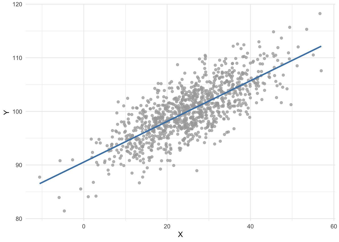
For instance, suppose we would like to estimate the relationship between two quantitative variables, \(X\) and \(Y\). Using the ordinary least squares method (the most common estimator used in linear regression), we obtain the following regression line:
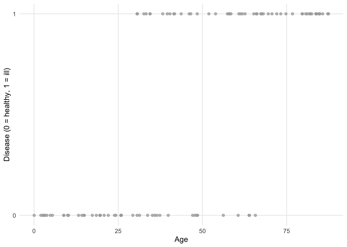
Now suppose we are interested in estimating the impact of age on whether or not a patient has a certain disease. Age is considered as a quantitative continuous variable, while having the disease is binary (a patient is either ill or healthy).
Visually, we could have something like this:
If we fit a regression line (using the ordinary least square method) to the points, we obtain the following plot:
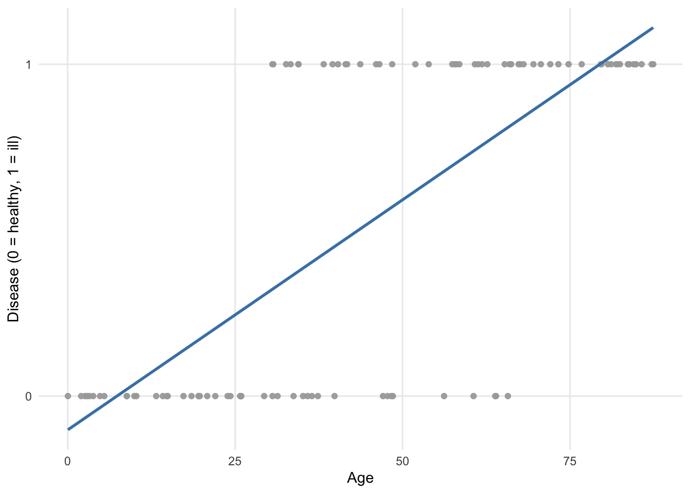
We see that the regression line goes below 0 and above 1 with respect to the \(y\)-axis. Since the dependent variable disease cannot take values below 0 (= healthy) nor above 1 (= ill), it is obvious that a linear regression is not appropriate for these data!
In addition to this limitation, the assumptions of normality and homoscedasticity, which are required in linear regression, are clearly not appropriate with these data since the dependent variable is binary and follows a Binomial distribution! R will not stop you from performing a linear regression on binary data, but this will produce a model of little interest.
This is where a logistic regression becomes handy as it takes into consideration these limitations.
Applied to our example, here is how the points are fitted using a binary logistic regression:
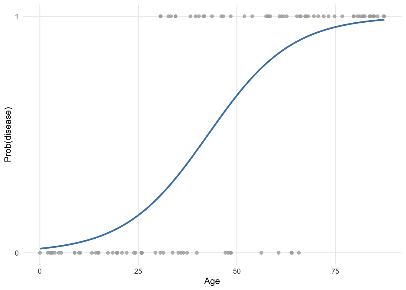
It is clear that this model is more appropriate.
The curve (known as a sigmoid) is obtained via a transformation of the predicted values. There are several possible choices for the link function, which aim is to constrain predicted values to be within the range of observed values.
The most widely used in practice is the logit function, which relates the probability of occurrence of an event (bounded between 0 and 1) to the linear combination of independent variables. The logit function also turns out to be the canonical link function for a Bernoulli or Binomial distribution. This transformation ensures that no matter in which range the \(X\) values are located, \(Y\) will only take numbers between 0 and 1.
One could say that the fitted values (= represented by the blue curve) taking values between 0 and 1 also does not seem to make sense since a patient can only be healthy or ill (and thus the dependent variable can only take the value 0 or 1, respectively). However, in a binary logistic regression it is not the outcome no disease/disease that is directly modeled, but the likelihood that a patient has the disease or not given his or her characteristics. This likelihood will be framed in terms of a probability to observe or not the disease in a patient, which is indeed included between 0 and 1, or 0% and 100%.
More generally, with a logistic regression we would like to model how the probability of success varies with the independent variables and determine whether or not these changes are statistically significant. We are actually going to model the logarithm of the odds, and the logistic regression model will be written as follows:
\[\begin{align} \log(odds(success)) &= logit(\pi) \\ &= \log\left(\frac{\pi}{1 - \pi}\right) \\ &= \beta_0 + \beta_1 X_1 + \cdots + \beta_p X_p \end{align}\]
where \(\pi\) \((0 \le \pi \le 1)\) is the probability of an event happening (success) and denoted \(\pi = P(success)\). We find the values of \(\hat{\beta}_0\), \(\hat{\beta}_1\), \(\ldots\), \(\hat{\beta}_p\), which are used as estimates for \(\beta_0\), \(\beta_1\), \(\ldots\), \(\beta_p\), using the maximum likelihood method. This method is one of several methods used in statistics to estimate parameters of a mathematical model. The goal of the estimator is to estimate the parameters \(\beta_0\), \(\beta_1\), \(\ldots\), \(\beta_p\) which maximize the log likelihood function. Different algorithms have been established over the years for this non-linear optimization, but this is beyond the scope of the post.
Logistic regressions are very common in the medical field, for example to:
- estimate the risk factors associated with a disease or a harmful condition,
- predict the risk of developing a disease based on a patient’s characteristics, or
- determine the most important biological factors associated with a specific disease or condition.
However, logistic regressions are used in many other domains, for instance in:
- banking sector: estimate a debtor’s creditworthiness based on his or her profile (income, assets, liabilities, etc.),
- marketing: estimate a customer’s propensity to buy a product or service based on his or her profile (age, sex, salary, previous purchases, etc.),
- sports: estimate the probability of a player winning against another player as a function of the characteristics of the two opponents,
- politics: answer the question “Would a citizen vote for our political party at the next elections?”
- etc.
Univariable versus multivariable logistic regression
Now that it is more clear when a binary logistic regression should be used, we show how to perform one in R. We start by presenting univariable binary logistic regressions, and then multivariable binary logistic regressions.
Remember that in both cases, the dependent variable must be a qualitative variable with two outcomes (hence the name binary logistic regression). The difference between a univariable and multivariable binary logistic regression lies in the fact that:
- for a univariable binary logistic regression, there is only one independent variable, while
- for a multivariable binary logistic regression, there are two ore more independent variables.
It is true that the term “univariable” may be confusing here because there are two variables in the model (i.e., one dependent variable and one independent variable). However, it is called univariable binary logistic regression to indicate that only one independent variable is considered in the model, as opposed to multivariable binary logistic regression where several independent variables are considered in the model.
To draw a parallel with linear regression:
- a univariable binary logistic regression is the equivalent of a simple linear regression, whereas
- a multivariable binary logistic regression is the equivalent of a multiple linear regression
when the dependent variable is binary instead of quantitative continuous. This is the reason a univariable binary logistic regression is sometimes called a simple binary logistic regression and a multivariable binary logistic regression sometimes called a multiple binary logistic regression.
The terms univariable/multivariable should not be confused with univariate/multivariate. The number of dependent variables characterizes the model as univariate or multivariate; univariate refers to a model with only one dependent variable, while multivariate refers to a model that simultaneously predicts more than one dependent variable. Usually, the intent is to differentiate models based on the number of independent variables. This distinction is made thanks to the terms univariable and multivariable. Multivariable refers to a model relating multiple predictor variables to a dependent variable, whereas univariable refers to a model relating one single independent variable to a dependent variable.
Data
For these illustrations, we use the “Heart Disease” dataset, available from the {kmed} R package. This data frame consists of 14 variables, of which only 5 of them are kept for this post:
age: age in yearssex: sex (FALSE = female, TRUE = male)cp: chest pain type (1 = typical angina, 2 = atypical angina, 3 = non-anginal pain, 4 = asymptomatic)thalach: maximum heart rate achievedclass: diagnosis of heart disease (divided into 4 classes)
# import and rename dataset
library(kmed)
dat <- heart

# select variables
library(dplyr)
dat <- dat |>
  select(
    age,
    sex,
    cp,
    thalach,
    class
  )

# print dataset's structure
str(dat)
## 'data.frame': 297 obs. of 5 variables:
## $ age : num 63 67 67 37 41 56 62 57 63 53 ...
## $ sex : logi TRUE TRUE TRUE TRUE FALSE TRUE ...
## $ cp : Factor w/ 4 levels "1","2","3","4": 1 4 4 3 2 2 4 4 4 4 ...
## $ thalach: num 150 108 129 187 172 178 160 163 147 155 ...
## $ class : int 0 2 1 0 0 0 3 0 2 1 ...
## - attr(*, "na.action")= 'omit' Named int [1:6] 88 167 193 267 288 303
## ..- attr(*, "names")= chr [1:6] "88" "167" "193" "267" ...Note that the pipe operator |> and the {dplyr} package is used to select variables. See more data manipulation techniques using this package if you are interested.
For greater readability, we rename the variables cp, thalach and class with more informative names:
# rename variables
dat <- dat |>
  rename(
    chest_pain = cp,
    max_heartrate = thalach,
    heart_disease = class
  )
We transform the variables sex and chest_pain into factor and set the labels accordingly:
# recode sex
dat$sex <- factor(dat$sex,
  levels = c(FALSE, TRUE),
  labels = c("female", "male")
)

# recode chest_pain
dat$chest_pain <- factor(dat$chest_pain,
  levels = 1:4,
  labels = c("typical angina", "atypical angina", "non-anginal pain", "asymptomatic")
)
For a binary logistic regression in R, it is recommended that all the qualitative variables are transformed into factors.
In our case, heart_disease (our dependent variable) is currently encoded as integer with values ranging from 0 to 4. Therefore, we first classify it into 2 classes by setting 0 for 0 values and 1 for non-0 values, using the ifelse() function:
# recode heart_disease into 2 classes
dat$heart_disease <- ifelse(dat$heart_disease == 0,
  0,
  1
)
We then transform it into a factor and set the labels accordingly using the factor() function:
# set labels for heart_disease
dat$heart_disease <- factor(dat$heart_disease,
  levels = c(0, 1),
  labels = c("no disease", "disease")
)
Keep in mind the order of the levels for your dependent variable, as it will have an impact on the interpretations. In R, the first level given by levels() is always taken as the reference level.
In our case, the first level is the absence of the disease and the second level is the presence of the disease:
levels(dat$heart_disease)## [1] "no disease" "disease"This means that when we will build the models, we will estimate the impact of the independent variable(s) on the presence of the disease (and not the absence!).
This is the reason that, for dependent variables of the type no/yes, false/true, absence/presence of a condition, etc. it is recommended to set the level no, false, absence of the condition, etc. as the reference level. It is indeed usually easier to interpret the impact of an independent variable on the presence of a condition/disease than the opposite.
If you want to switch the reference level, this can be done with the relevel() function.
Here is a preview of the final data frame and some basic descriptive statistics:
# print first 6 observations
head(dat)
## age sex chest_pain max_heartrate heart_disease
## 1 63 male typical angina 150 no disease
## 2 67 male asymptomatic 108 disease
## 3 67 male asymptomatic 129 disease
## 4 37 male non-anginal pain 187 no disease
## 5 41 female atypical angina 172 no disease
## 6 56 male atypical angina 178 no disease# basic descriptive statistics
summary(dat)## age sex chest_pain max_heartrate
## Min. :29.00 female: 96 typical angina : 23 Min. : 71.0
## 1st Qu.:48.00 male :201 atypical angina : 49 1st Qu.:133.0
## Median :56.00 non-anginal pain: 83 Median :153.0
## Mean :54.54 asymptomatic :142 Mean :149.6
## 3rd Qu.:61.00 3rd Qu.:166.0
## Max. :77.00 Max. :202.0
## heart_disease
## no disease:160
## disease :137
##
##
##
## The data frame is now ready to be analyzed further through univariable and multivariable binary logistic regressions.
Binary logistic regression in R
Univariable binary logistic regression
As mentioned above, we start with a univariable binary logistic regression, that is, a binary logistic regression with only one independent variable.
In R, a binary logistic regression can be done with the glm() function and the family = "binomial" argument. Similar to linear regression, the formula used inside the function must be written as dependent variable ~ independent variable (in this order!).
While the dependent variable must be categorical with two levels, the independent variable can be of any type. However, interpretations differ depending on whether the independent variable is qualitative or quantitative.
For completeness, we illustrate this type of regression with both a quantitative and a qualitative independent variable, starting with a quantitative independent variable.
Quantitative independent variable
Suppose we want to estimate the impact of a patient’s age on the presence of heart disease. In this case, age is our independent variable and heart_disease is our dependent variable:
# save model
m1 <- glm(heart_disease ~ age,
  data = dat,
  family = "binomial"
)
Results of the model is saved under the object m1. Again, similar to linear regression, results can be accessed thanks to the summary() function:
# print results
summary(m1)
##
## Call:
## glm(formula = heart_disease ~ age, family = "binomial", data = dat)
##
## Coefficients:
## Estimate Std. Error z value Pr(>|z|)
## (Intercept) -3.05122 0.76862 -3.970 7.2e-05 ***
## age 0.05291 0.01382 3.829 0.000128 ***
## ---
## Signif. codes: 0 '***' 0.001 '**' 0.01 '*' 0.05 '.' 0.1 ' ' 1
##
## (Dispersion parameter for binomial family taken to be 1)
##
## Null deviance: 409.95 on 296 degrees of freedom
## Residual deviance: 394.25 on 295 degrees of freedom
## AIC: 398.25
##
## Number of Fisher Scoring iterations: 4The most important results in this output are displayed in the table after Coefficients. The bottom part of the output summarizes the distribution of the deviance residuals. In a nutshell, deviance residuals measure how well the observations fit the model. The closer the residual to 0, the better the fit of the observation.
Within the Coefficients table, we focus on the first and last columns (the other two columns correspond to the standard error and the test statistic, which are both used to compute the \(p\)-value):
- the column
Estimatecorresponds to the coefficients \(\hat{\beta}_0\) and \(\hat{\beta}_1\), and - the column
Pr(>|z|)corresponds to the \(p\)-values.
R performs a hypothesis test for each coefficient, that is, \(H_0: \beta_j = 0\) versus \(H_1: \beta_j \neq 0\) for \(j = 0, 1\) via the Wald test, and print the \(p\)-values in the last column. We can thus compare these \(p\)-values to the chosen significance level (usually \(\alpha = 0.05\)) to conclude whether or not each of the coefficient is significantly different from 0. The lower the \(p\)-value, the more evidence that the coefficient is different from 0. This is similar to linear regression.
Coefficients are slightly harder to interpret in logistic regression than in linear regression because the relationship between dependent and independent variables is not linear.
Let’s first interpret the coefficient of age, \(\hat{\beta}_1\), which is the most important coefficient of the two.
First, since the \(p\)-value of the test on the coefficient for age is < 0.05, we conclude that it is significantly different from 0, which means that age is significantly associated with the presence of heart disease (at the 5% significance level). Note that if the test was not significant (i.e., the \(p\)-value \(\ge \alpha\)), we would refrain from interpreting the coefficient since it means that, based on the data at hand, we are unable to conclude that age is associated with the presence of heart disease in the population.
Second, remember that:
- when \(\beta_1 = 0\), \(X\) and \(Y\) are independent,
- when \(\beta_1 > 0\), the probability that \(Y = 1\) increases with \(X\), and
- when \(\beta_1 < 0\), the probability that \(Y = 1\) decreases with \(X\).
In our context, we have:
- when \(\hat{\beta}_1 = 0\), the probability of developing a heart disease is independent of the age,
- when \(\hat{\beta}_1 > 0\), the probability of developing a heart disease increases with age, and
- when \(\hat{\beta}_1 < 0\), the probability of developing a heart disease decreases with age.
Here we have \(\hat{\beta}_1 =\) 0.053 \(> 0\), so we already know that the older the patient, the more likely he or she is to develop a heart disease. This makes sense.
Now that we know the direction of the relationship, we would like to quantify this relationship. This is easily done thanks to odds ratios (OR). OR are found by taking the exponential of the coefficients. In R, the exponential is done thanks to the exp() function.
OR can be interpreted as follows: the OR is the multiplicative change in the odds in favor of \(Y = 1\) when \(X\) increases by 1 unit.
Applied to our context, we compute the OR for the age by computing \(\exp(\hat{\beta}_1) =\) exp(0.053).
Using R, this gives:
# OR for age
exp(coef(m1)["age"])
## age
## 1.054331Based on this result, we can say that an extra year of age increases the odds (that is, the chance) of developing a heart disease by a factor of 1.054.
Therefore, the odds of developing a heart disease increases by (1.054 - 1) \(\times\) 100 = 5.4% when a patient becomes one year older.
To sum up:
- when the coefficient \(\hat{\beta}_1 = 0 \Rightarrow\) OR \(= \exp(\hat{\beta}_1) = 1 \Rightarrow P(Y = 1)\) is independent of \(X \Rightarrow\) there is no relationship between \(X\) and \(Y\),
- when the coefficient \(\hat{\beta}_1 > 0 \Rightarrow\) OR \(= \exp(\hat{\beta}_1) > 1 \Rightarrow P(Y = 1)\) increases with \(X \Rightarrow\) there is a positive relationship between \(X\) and \(Y\), and
- when the coefficient \(\hat{\beta}_1 < 0 \Rightarrow\) OR \(= \exp(\hat{\beta}_1) < 1 \Rightarrow P(Y = 1)\) decreases with \(X \Rightarrow\) there is a negative relationship between \(X\) and \(Y\).
We now interpret the intercept \(\hat{\beta}_0\).
First, we look at the \(p\)-value of the test on the intercept. This \(p\)-value being < 0.05, we conclude that the intercept is significantly different from 0 (at the 5% significance level).
Second, similar to linear regression, in order to obtain an interpretation of the intercept, we need to find a situation in which the other coefficient, \(\beta_1\), vanishes.
In our case, it happens when a patient is 0 year old. We may or may not need to interpret results in a such a situation, and in many situations the interpretation does not make sense, so it is more a hypothetical interpretation. However, again for completeness we show how to interpret the intercept. Note that it is also possible to center the numeric variable so that the intercept has a more meaningful interpretation. This, however, goes beyond the scope of the post.
For a patient aged 0 year, the odds of developing a heart disease is \(\exp(\hat{\beta}_0) =\) exp(-3.051) = 0.047. When interpreting an intercept, it often makes more sense to interpret it as the probability that \(Y = 1\), which can be computed as follows:
\[\frac{\exp(\hat{\beta}_0)}{1 + \exp(\hat{\beta}_0)}.\]
In our case, it corresponds to the probability that a patient of age 0 develops a heart disease, which is equal to:
# prob(heart disease) for age = 0
exp(coef(m1)[1]) / (1 + exp(coef(m1)[1]))
## (Intercept)
## 0.04516478This means that, if we trust our model, a newborn is expected to develops a heart disease with a probability of 4.52%.
For your information, a confidence interval can be computed for any of the OR using the confint() function. For example, a 95% confidence interval for the OR for age:
# 95% CI for the OR for age
exp(confint(m1,
  parm = "age"
))
## 2.5 % 97.5 %
## 1.026699 1.083987Remember than when evaluating an OR, the null value is 1, not 0. An OR of 1 in this study would mean that there is no association between the age and the presence of heart disease. If the 95% confidence interval of the OR does not include 1, we conclude that there is a significant association between the age and the presence of heart disease. On the contrary, if it includes 1, we do not reject the hypothesis that there is no association between age and the presence of heart disease.
In our case, the 95% CI does not include 1, so we conclude, at the 5% significance level, that there is a significant association between age and the presence of heart disease.
You will notice that it is the same conclusion than with the \(p\)-value. This is normal, it will always be the case:
- if the \(p\)-value < 0.05, 1 will not be included in the 95% CI, and
- if the \(p\)-value \(\ge\) 0.05, 1 will be included in the 95% CI.
This means that you can choose whether you draw your conclusion about the association between the two variables based on the 95% CI or the \(p\)-value.
Estimating the relationship between variables is the main reason for building models. Another goal is to predict the dependent variable based on newly observed values of the independent variable(s). This can be done with the predict() function.
Suppose we would like to predict the probability of developing a heart disease for a patient aged 30 years old:
# predict probability to develop heart disease
pred <- predict(m1,
  newdata = data.frame(age = c(30)),
  type = "response"
)

# print prediction
pred
## 1
## 0.1878525It is predicted that a 30-year-old patient has a 18.79% chance of developing a heart disease.
Note that if you would like to construct a confidence interval for this prediction, it can be done by adding the se = TRUE argument in the predict() function:
# predict probability to develop heart disease
pred <- predict(m1,
  newdata = data.frame(age = c(30)),
  type = "response",
  se = TRUE
)

# print prediction
pred$fit
## 1
## 0.1878525# 95% confidence interval for the prediction
lower <- pred$fit - (qnorm(0.975) * pred$se.fit)
upper <- pred$fit + (qnorm(0.975) * pred$se.fit)
c(lower, upper)## 1 1
## 0.07873357 0.29697138If you are a frequent reader of the blog, you are probably know that I like visualizations. The plot_model() function available in the {sjPlot} R package does a good job of visualizing results of the model:
# load package
library(sjPlot)

# plot
plot_model(m1,
  type = "pred",
  terms = "age"
) +
  labs(y = "Prob(heart disease)")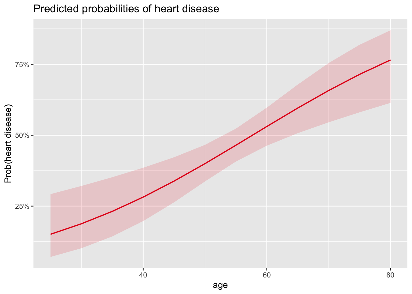
For those of you who are familiar with the {ggplot2} package, you will have noticed that the function accepts layers from the {ggplot2} package. Note also that this function works with other types of model (such as linear models).
The above plot shows the probability of developing a heart disease in function of age, and confirms results found above:
- We see that the probability of developing a heart disease increases with age (which was expected given that the OR for the coefficient of age is > 1),
- and we also see that the probability of developing a heart disease for a 30-year-old patient is slightly below 20%.
Qualitative independent variable
Suppose now that we are interested in estimating the relationship between the probability of developing a heart disease and the sex (which is a qualitative variable).
Recall that when the independent variable was quantitative, \(\exp(\hat{\beta}_1)\) was the multiplicative change in the odds in favor of \(Y = 1\) as \(X\) increases by 1 unit.
With \(X\) being the sex, the only unit increase possible is from 0 to 1 (or from 1 to 2 if sex is encoded as a factor), so we can write an interpretation in terms of female/male:
- \(\exp(\hat{\beta}_1)\) is the multiplicative change of the odds in favor of \(Y = 1\) as a female becomes a male.
Again, keep in mind what is the order of the level for the variable sex. In our case, the level female comes before the level male:
# levels for sex
levels(dat$sex)
## [1] "female" "male"So it is indeed the multiplicative change of the odds in favor of \(Y = 1\) as a female becomes a male. If the level male came before the level female in our dataset, it would have been the opposite.
You will concede that it is rather strange to interpret odds as a female becomes a male, or vice versa. Therefore, it is better to say:
- \(\exp(\hat{\beta}_1)\) is the multiplicative change of the odds in favor of \(Y = 1\) for males versus females.
In our case, we obtain the following results:
# save model
m2 <- glm(heart_disease ~ sex,
  data = dat,
  family = "binomial"
)

# print results
summary(m2)
##
## Call:
## glm(formula = heart_disease ~ sex, family = "binomial", data = dat)
##
## Coefficients:
## Estimate Std. Error z value Pr(>|z|)
## (Intercept) -1.0438 0.2326 -4.488 7.18e-06 ***
## sexmale 1.2737 0.2725 4.674 2.95e-06 ***
## ---
## Signif. codes: 0 '***' 0.001 '**' 0.01 '*' 0.05 '.' 0.1 ' ' 1
##
## (Dispersion parameter for binomial family taken to be 1)
##
## Null deviance: 409.95 on 296 degrees of freedom
## Residual deviance: 386.12 on 295 degrees of freedom
## AIC: 390.12
##
## Number of Fisher Scoring iterations: 4# OR for sex
exp(coef(m2)["sexmale"])## sexmale
## 3.573933which can be interpreted as follows:
- The \(p\)-value of the test on the coefficient for sex is < 0.05, so we conclude that the sex is significantly associated with the presence of heart disease (at the 5% significance level).
- Moreover, when looking at the coefficient for sex, \(\hat{\beta}_1 =\) 1.274, we can say that:
- For males, the odds of developing a heart disease is multiplied by a factor of exp(1.274) = 3.574 compared to females.
- In other words, the odds of developing a heart disease for males are 3.574 times the odds for females.
- This means that, the odds of developing a heart disease are (3.574 - 1) \(\times\) 100 = 257.4% higher for males than for females.
These results again make sense, as it known that men are more likely to have a heart disease than women.
The interpretation of the intercept \(\hat{\beta}_0 =\) -1.044 is similar than in the previous section in the sense that it gives the probability of developing a heart disease when the other coefficient, \(\beta_1\), is equal to 0.
In our case, \(\beta_1 = 0\) simply means that the patient is a female. Therefore, the probability of developing a heart disease for a woman is:
# prob(disease) for sex = female
exp(coef(m2)[1]) / (1 + exp(coef(m2)[1]))
## (Intercept)
## 0.2604167The avid reader will notice that a univariable binary logistic regression with a qualitative independent variable will lead to the same conclusion than a Chi-square test of independence:
chisq.test(table(dat$heart_disease, dat$sex))##
## Pearson's Chi-squared test with Yates' continuity correction
##
## data: table(dat$heart_disease, dat$sex)
## X-squared = 21.852, df = 1, p-value = 2.946e-06Based on this test, we reject the null hypothesis of independence between the two variables and we thus conclude that there is a significant association between the sex and the presence of heart disease (\(p\)-value < 0.001).
The advantage of a univariable binary logistic regression over a Chi-square test of independence is that it not only tests whether or not there is a significant association between the two variables, but it also estimates the direction and strength of this relationship.
As for a univariable logistic regression with a quantitative independent variable, predictions can also be made with the predict() function. Suppose we would like to predict the probability of developing a heart disease for a male:
# predict probability to develop heart disease
pred <- predict(m2,
  newdata = data.frame(sex = c("male")),
  type = "response"
)

# print prediction
pred
## 1
## 0.5572139Based on this model, it is predicted that a male patient has 55.72% chance of developing a heart disease.
We can also visualize these results thanks to the plot_model() function:
# plot
plot_model(m2,
  type = "pred",
  terms = "sex"
) +
  labs(y = "Prob(heart disease)")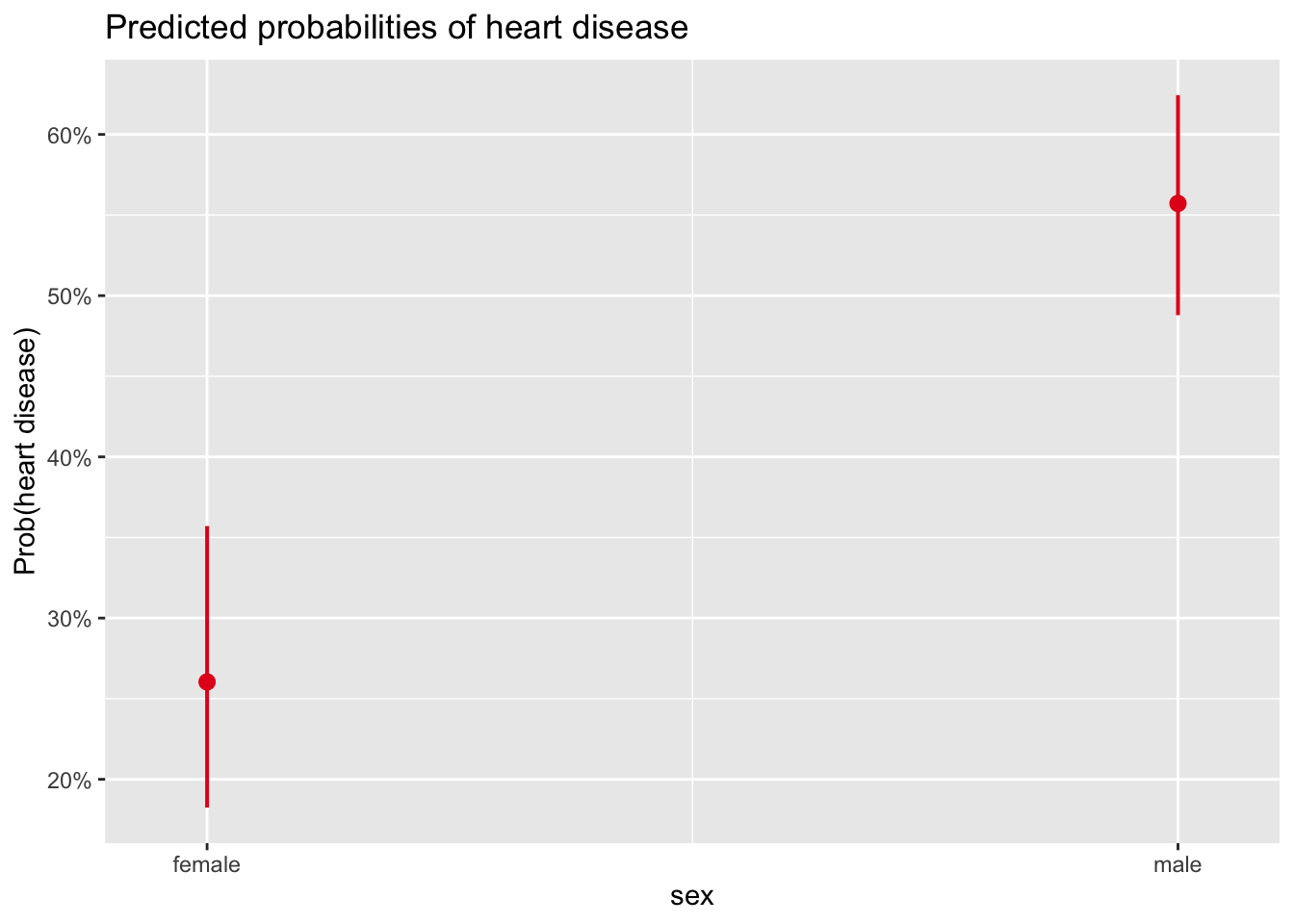
The points correspond to the predicted probabilities, and the bars correspond to their confidence intervals.
The plot of the results in terms of probabilities confirms what was found above, that is:
- women are less likely to develop a heart disease than men,
- the probability that a woman develops a heart disease is expected to be slightly above 25%, and
- the probability that a man develops a heart disease is expected to be around 55%.
Multivariable binary logistic regression
The interpretation of the coefficients in multivariable logistic regression is similar to the interpretation in univariable regression, except that this time it estimates the multiplicative change in the odds in favor of \(Y = 1\) when \(X\) increases by 1 unit, while the other independent variables remain unchanged.
This is similar to multiple linear regression, where a coefficient gives the expected change of \(Y\) for an increase of 1 unit of \(X\), while keeping all other variables constant.
The main advantages of using a multivariable logistic regression compared to a univariable logistic regression are to:
- consider the simultaneous (rather than isolated) effect of independent variables,
- take into account potential confounding and/or interaction effects, and
- improve predictions.
For this illustration, suppose we would like to estimate the relationship between heart disease and all variables present in the data frame, that is, age, sex, chest pain type and maximum heart rate achieved:
# save model
m3 <- glm(heart_disease ~ .,
  data = dat,
  family = "binomial"
)

# print results
summary(m3)
##
## Call:
## glm(formula = heart_disease ~ ., family = "binomial", data = dat)
##
## Coefficients:
## Estimate Std. Error z value Pr(>|z|)
## (Intercept) -0.060150 1.962091 -0.031 0.975544
## age 0.042814 0.019009 2.252 0.024302 *
## sexmale 1.686330 0.349352 4.827 1.39e-06 ***
## chest_painatypical angina -0.120481 0.641396 -0.188 0.851000
## chest_painnon-anginal pain -0.124331 0.571093 -0.218 0.827658
## chest_painasymptomatic 1.963723 0.548877 3.578 0.000347 ***
## max_heartrate -0.030326 0.007975 -3.802 0.000143 ***
## ---
## Signif. codes: 0 '***' 0.001 '**' 0.01 '*' 0.05 '.' 0.1 ' ' 1
##
## (Dispersion parameter for binomial family taken to be 1)
##
## Null deviance: 409.95 on 296 degrees of freedom
## Residual deviance: 275.26 on 290 degrees of freedom
## AIC: 289.26
##
## Number of Fisher Scoring iterations: 5Note that the formula heart_disease ~ . is a shortcut to include all variables present in the data frame in the model as independent variables, except heart_disease.
Based on the \(p\)-values displayed in the last column of the coefficients table, we conclude that, at the 5% significance level, age, sex and maximum heart rate achieved are all significantly associated with heart disease (\(p\)-values < 0.05).
For the variables age, sex and max_heartrate, there is only one \(p\)-value (the result of the test on the nullity of the coefficient).
For the variable chest_pain, 3 \(p\)-values are displayed. This is normal: similar to linear regression when a categorical variable with more than two levels is included in the model, one test is performed for each comparison between the reference level and the other levels.
In our case, the reference level for the variable chest_pain is typical angina as it comes first:
levels(dat$chest_pain)## [1] "typical angina" "atypical angina" "non-anginal pain" "asymptomatic"Therefore, a test is performed for the comparison between:
typical anginaandatypical angina,typical anginaandnon-anginal pain, andtypical anginaandasymptomatic.
But here we are not interested in comparing levels of the variable chest pain, we would like to test the overall effect of chest pain on heart disease. For this, we are going to compare two models via a likelihood ratio test (LRT):
- a model which includes all the variables of interest and the variable
chest_pain, and - the exact same model but which excludes the variable
chest_pain.
The first one is referred as the full or complete model, whereas the second one is referred as the reduced model.
We compare these two models with the anova() function:
# save reduced model
m3_reduced <- glm(heart_disease ~ age + sex + max_heartrate,
  data = dat,
  family = "binomial"
)

# compare reduced with full model
anova(m3_reduced, m3,
  test = "LRT"
)
## Analysis of Deviance Table
##
## Model 1: heart_disease ~ age + sex + max_heartrate
## Model 2: heart_disease ~ age + sex + chest_pain + max_heartrate
## Resid. Df Resid. Dev Df Deviance Pr(>Chi)
## 1 293 325.12
## 2 290 275.26 3 49.86 8.558e-11 ***
## ---
## Signif. codes: 0 '***' 0.001 '**' 0.01 '*' 0.05 '.' 0.1 ' ' 1Notice that the reduced model must come before the complete model in the anova() function. The null hypothesis of this test is that the two models are equivalent.
At the 5% significance level (see the \(p\)-value at the right of the R output), we reject the null hypothesis and we conclude that the complete model is significantly better than the reduced model at explaining the presence of heart disease. This means that chest pain is significantly associated with heart disease (which was expected since the comparison between typical angina and asymptomatic was found to be significant).
A comparison of two models via the LRT will be shown again later, when discussing about interactions.
Now that we have shown that all four independent variables were significantly associated with the presence of heart disease, we can interpret the coefficients in order to know the direction of the relationships and most importantly, quantify the strength of these relationships.
Like univariable binary logistic regression, it is easier to interpret these relationships through OR. But this time, we also print the 95% CI of the OR in addition to the OR (rounded to 3 decimals) so that we can easily see which ones are significantly different from 1:
# OR and 95% CI
round(exp(cbind(OR = coef(m3), confint(m3))), 3)
## OR 2.5 % 97.5 %
## (Intercept) 0.942 0.020 44.353
## age 1.044 1.006 1.084
## sexmale 5.400 2.776 10.971
## chest_painatypical angina 0.886 0.252 3.191
## chest_painnon-anginal pain 0.883 0.293 2.814
## chest_painasymptomatic 7.126 2.509 22.030
## max_heartrate 0.970 0.955 0.985From the OR and their 95% CI computed above, we conclude that:
- Age: the odds of having a heart disease are multiplied by a factor of 1.04 for each one-unit increase in age, all else being equal.
- Sex: the odds of developing a heart disease for males are 5.4 times the odds for females, all else being equal.
- Chest pain: the odds of developing a heart disease for people suffering from chest pain of the type “asymptomatic” are 7.13 times the odds for people suffering from chest pain of the type “typical angina”, all else being equal. We refrain from interpreting the other comparisons as they are not significant at the 5% significance level (1 is included in their 95% CI).
- Maximum heart rate achieved: the odds of having a heart disease are multiplied by a factor of 0.97 for each one-unit increase in maximum heart rate achieved, all else being equal.
- Intercept: we also refrain from interpreting the intercept as it is not significantly different from 0 at the 5% significance level (1 is included in the 95% CI).
If you are interested in printing only the OR for which the \(p\)-value of the coefficient is < 0.05, here is the code:
exp(coef(m3))[coef(summary(m3))[, "Pr(>|z|)"] < 0.05]## age sexmale chest_painasymptomatic
## 1.0437437 5.3996293 7.1258054
## max_heartrate
## 0.9701289Remember that we can always write the interpretations in terms of the percentage increase/decrease in odds with the formula \((OR - 1) \times 100\), where OR corresponds to the odds ratio.
For instance, for the maximum heart rate achieved, the OR = 0.97, so the interpretation becomes: the odds of developing a heart disease increases by (0.97 \(- 1) \times 100 =\) -3% for each one-unit increase in maximum heart rate achieved, which is equivalent to say that the odds of developing a heart disease decreases by 3% for each one-unit increase in maximum heart rate achieved.
For illustrative purposes, suppose now that we would like to predict the probability that a new patient develops a heart disease. Suppose that this patient is a 32-year-old woman, suffering from chest pain of the type non-anginal and she achieved a maximum heart rate of 150. The probability that she develops a heart disease is:
# create data frame of new patient
new_patient <- data.frame(
  age = 32,
  sex = "female",
  chest_pain = "non-anginal pain",
  max_heartrate = 150
)

# predict probability to develop heart disease
pred <- predict(m3,
  newdata = new_patient,
  type = "response"
)

# print prediction
pred
## 1
## 0.03345948If we trust our model, the probability that this new patient will develop a heart disease is predicted to be 3.35%.
We can also visualize the results thanks to the plot_model() function, three effects at the same time:
- effect of age, sex and chest pain type on the predicted probability of developing a heart disease, and
- effect of maximum heart rate achieved, sex and chest pain type on the predicted probability of developing a heart disease.
# 1. age, sex and chest pain on prob of disease
plot_model(m3,
  type = "pred",
  terms = c("age", "chest_pain", "sex"),
  ci.lvl = NA # remove confidence bands
) +
  labs(y = "Prob(heart disease)")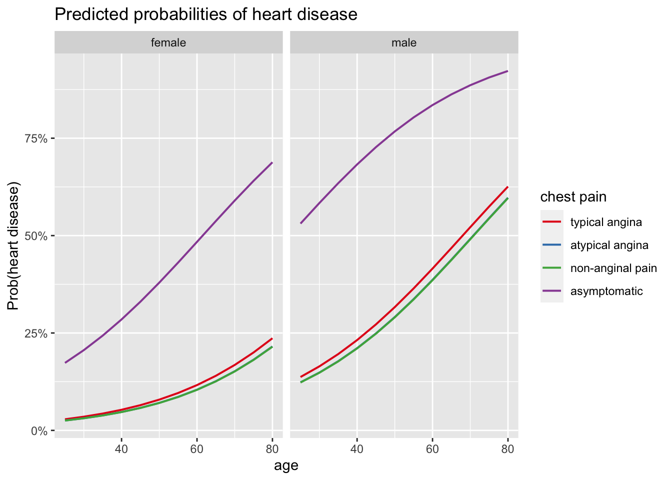
# 2. max heart rate, chest pain and sex on prob of disease
plot_model(m3,
  type = "pred",
  terms = c("max_heartrate", "chest_pain", "sex"),
  ci.lvl = NA # remove confidence bands
) +
  labs(y = "Prob(heart disease)")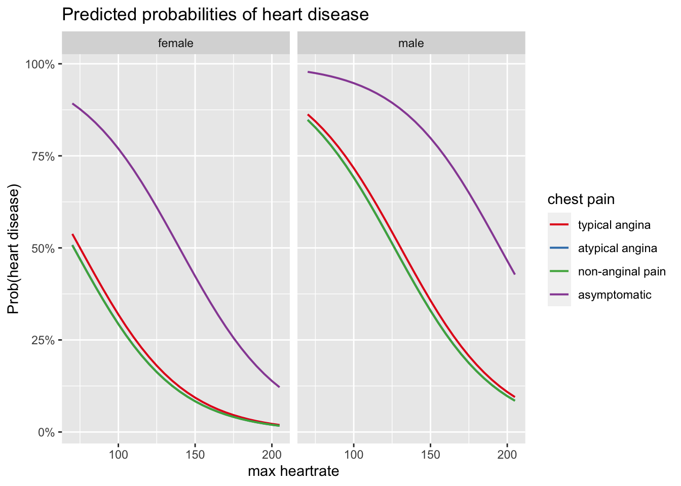
For more clarity in the plots, confidence bands are removed thanks to ci.lvl = NA.
These plots confirm results obtained above, that is:
- there is a positive relationship between age and the presence of heart disease,
- there is a negative relationship between maximum heart rate achieved and the presence of heart disease,
- the odds of developing a heart disease is higher for patients suffering from chest pain of the type asymptomatic and similar for the 3 other types of chest pain, and
- the odds of developing a heart disease is higher for males than for females.
Interaction
In the previous sections, potential interaction effects were omitted.
An interaction occurs when the relationship between an independent variable and the outcome variable depends on the value or the level taken by another independent variable. On the contrary, if the relationship between an independent variable and the dependent variable remains unchanged no matter the value taken by another independent variable, we cannot conclude that there is an interaction effect.
In our case, there would be an interaction if for example the relationship between age and heart disease depends on the sex. There would be an interaction, for instance, if the relationship between age and heart disease was positive for females, and negative for males, or vice versa. Or if the relationship between age and heart disease was much stronger or much weaker for females than for males.
Let’s see if there is an interaction between age and sex, and more importantly, whether or not this interaction is significant. For this, we need to build two models:
- one model containing only the main effects, so without the interaction, and
- one model containing the main effects and the interaction.
# save model without interaction
m4 <- glm(heart_disease ~ age + sex,
  data = dat,
  family = "binomial"
)

# save model with interaction
m4_inter <- glm(heart_disease ~ age * sex,
  data = dat,
  family = "binomial"
)
We first assess the interaction visually via the plot_model() function:
# plot
plot_model(m4_inter,
  type = "pred",
  terms = c("age", "sex"),
  ci.lvl = NA # remove confidence bands
) +
  labs(y = "Prob(heart disease)")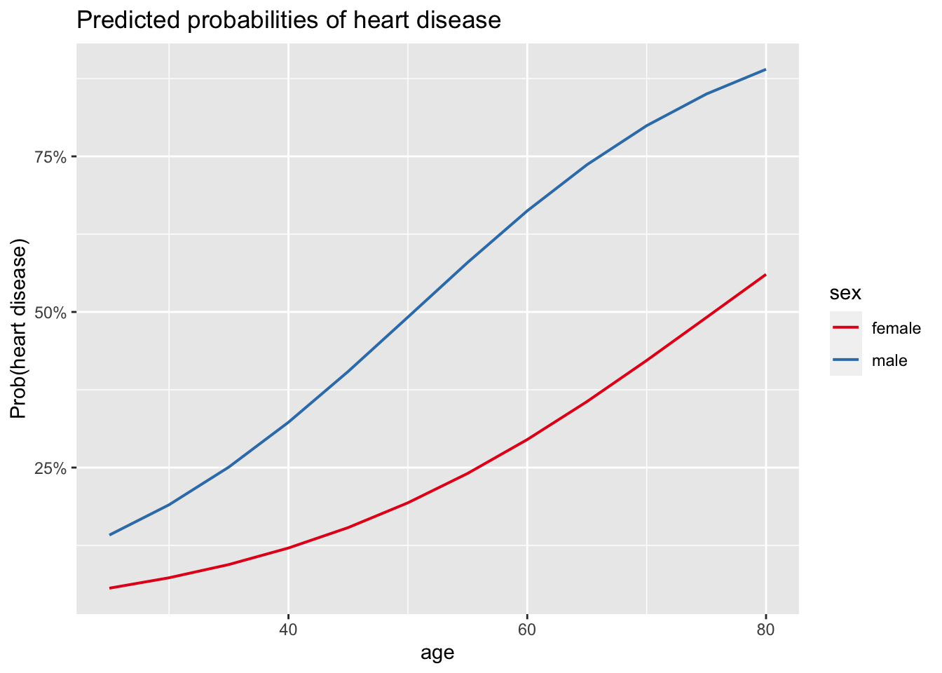
Since the two curves of the predicted probabilities are relatively similar and follow the same pattern, the relationship between age and the presence of heart disease does not seem to depend on the sex, indicating that there may indeed be no interaction. However, we would like to test it more formally via a statistical test.
For this, we can compare the two models (the one without compared to the one with interaction) with a likelihood ratio test (LRT), using the anova() function:
anova(m4, m4_inter,
  test = "LRT"
)
## Analysis of Deviance Table
##
## Model 1: heart_disease ~ age + sex
## Model 2: heart_disease ~ age * sex
## Resid. Df Resid. Dev Df Deviance Pr(>Chi)
## 1 294 364.43
## 2 293 364.23 1 0.20741 0.6488Remember that it is always the reduced model as the first argument in the anova() function, and then the more complex model as the second argument.
The test confirms what we supposed based on the plot: at the 5% significance level, we do not reject the null hypothesis that the two models are equivalent. Since the only difference between the two models is that an interaction term is added in the complete model, we do not reject the hypothesis that there is no interaction between the age and the sex (\(p\)-value = 0.649).
This conclusion could have also been obtained more simply with the drop1() function:
drop1(m4_inter,
  test = "LRT"
)
## Single term deletions
##
## Model:
## heart_disease ~ age * sex
## Df Deviance AIC LRT Pr(>Chi)
## <none> 364.23 372.23
## age:sex 1 364.43 370.43 0.20741 0.6488As you can see, this gives the same \(p\)-value of 0.649.
In practice, a non-significant interaction is removed from the model before interpreting its results. In our case, only the main effects of age and sex would remain in the model.
This leads us to model selection, or which variables should be included in our final model. This is discussed in the next section.
Model selection
In practice, we often have several models, corresponding to the different combinations of independent variables and their interactions. Finding the best model is not easy.
In general, the best practice is to obtain a final model that is as parsimonious as possible, that is, with as few parameters as possible. A parsimonious model is easier to interpret and generalize, and also more powerful from a statistical point of view. On the other hand, it should not be too simple so that it still captures the variations or patterns in the data. In general, while more variables are often better than one, too many is often worse than a few.
The two most common approaches to obtain a final model are the following:
- Adjust the model by removing the main effects and their interactions which are not significant with respect to their \(p\)-values, obtained by testing the nullity of the corresponding coefficients using a statistical test such as the likelihood ratio test or the Wald test. If there are several main effects or interactions which are not significant, interactions must be removed before removing any main effect. Moreover, it is recommended to remove interactions and independent variables one by one (starting with the one with the highest \(p\)-value), as removing a variable or an interaction may make another variable or interaction that was initially non-significant significant.
- Adjust the model by using AIC (Akaike Information Criterion) or BIC (Bayesian Information Criterion). These procedures allow to select the best model (according to AIC or BIC) by finding an equilibrium between simplicity and complexity. These selection processes usually lead to a final model with as few parameters as possible, but which captures as much information in the data as possible. Note that only models with the same dependent variable can be compared using AIC or BIC. Models with different dependent variables cannot be compared using these criteria.
The first method requires that:
- the underlying assumptions are valid,
- the sample size is sufficiently large, and
- the models are nested (i.e., the complete model includes at least all the variables included in the reduced model).
Moreover, the second method can be used with widely used criteria when selecting variables, and more importantly, in a completely autonomous way in R.
For this reason, the second method is recommended and more often used in practice.
This second method, referred as the stepwise selection, is divided into 3 types:
- backward selection: we start from the most complete model (containing all independent variables and usually also their interactions), and the interactions/main effects are deleted at each step until the model cannot be improved,
- forward selection: we start from the most basic model containing only the intercept, and the independent variables/interactions are added at each step until the model cannot be improved, or
- mixed selection: we apply both the backward and forward selection to determine the best model according to the desired criterion.
We show how to select the best model according to AIC using the mixed stepwise selection, illustrated with all variables present in the data frame as independent variables and all possible second order interactions:
# save initial model
m5 <- glm(heart_disease ~ (age + sex + chest_pain + max_heartrate)^2,
  data = dat,
  family = "binomial"
)

# select best model according to AIC using mixed selection
m5_final <- step(m5,
  direction = "both", # both = mixed selection
  trace = FALSE # do not display intermediate steps
)

# display results of final model
summary(m5_final)
##
## Call:
## glm(formula = heart_disease ~ age + sex + chest_pain + max_heartrate +
## age:max_heartrate, family = "binomial", data = dat)
##
## Coefficients:
## Estimate Std. Error z value Pr(>|z|)
## (Intercept) 19.4386591 8.1904201 2.373 0.017628 *
## age -0.3050017 0.1414986 -2.156 0.031122 *
## sexmale 1.7055353 0.3507149 4.863 1.16e-06 ***
## chest_painatypical angina -0.0086463 0.6547573 -0.013 0.989464
## chest_painnon-anginal pain -0.0590333 0.5844000 -0.101 0.919538
## chest_painasymptomatic 1.9724490 0.5649516 3.491 0.000481 ***
## max_heartrate -0.1605658 0.0540933 -2.968 0.002994 **
## age:max_heartrate 0.0023314 0.0009433 2.471 0.013457 *
## ---
## Signif. codes: 0 '***' 0.001 '**' 0.01 '*' 0.05 '.' 0.1 ' ' 1
##
## (Dispersion parameter for binomial family taken to be 1)
##
## Null deviance: 409.95 on 296 degrees of freedom
## Residual deviance: 268.60 on 289 degrees of freedom
## AIC: 284.6
##
## Number of Fisher Scoring iterations: 5According to the AIC (which is the default criterion when using the step() function), the best model is the one including:
age,sex,chest_pain,max_heartrate, and- the interaction between
ageandmax_heartrate.
For your information, you can also easily compare models manually using AIC or the pseudo-\(R^2\) with the tab_model() function, also available in the {sjPlot} R package:
tab_model(m3, m4, m5_final,
  show.ci = FALSE, # remove CI
  show.aic = TRUE, # display AIC
  p.style = "numeric_stars" # display p-values and stars
)| heart disease | heart disease | heart disease | ||||
|---|---|---|---|---|---|---|
| Predictors | Odds Ratios | p | Odds Ratios | p | Odds Ratios | p |
| (Intercept) | 0.94 | 0.976 | 0.01 *** | <0.001 | 276759408.51 * | 0.018 |
| age | 1.04 * | 0.024 | 1.07 *** | <0.001 | 0.74 * | 0.031 |
| sex [male] | 5.40 *** | <0.001 | 4.47 *** | <0.001 | 5.50 *** | <0.001 |
|
chest pain [atypical angina] |
0.89 | 0.851 | 0.99 | 0.989 | ||
|
chest pain [non-anginal pain] |
0.88 | 0.828 | 0.94 | 0.920 | ||
| chest pain [asymptomatic] | 7.13 *** | <0.001 | 7.19 *** | <0.001 | ||
| max heartrate | 0.97 *** | <0.001 | 0.85 ** | 0.003 | ||
| age × max heartrate | 1.00 * | 0.013 | ||||
| Observations | 297 | 297 | 297 | |||
| R2 Tjur | 0.393 | 0.142 | 0.409 | |||
| AIC | 289.263 | 370.435 | 284.599 | |||
|
||||||
Pseudo-\(R^2\) is a generalization of the coefficient of determination \(R^2\) often used in linear regression to judge the quality of a model. Like the \(R^2\) in linear regression, the pseudo-\(R^2\) varies from 0 to 1, and can be interpreted as the percentage of the null deviance explained by the independent variable(s). The higher the pseudo-\(R^2\) and the lower the AIC, the better the model.
Note that there are several pseudo-\(R^2\), such as:
- Likelihood ratio \(R^2_{L}\),
- Cox and Snell \(R^2_{CS}\),
- Nagelkerke \(R^2_{N}\),
- McFadden \(R^2_{McF}\), and
- Tjur \(R^2_{T}\).
The tab_model() function gives the Tjur \(R^2_{T}\) by default.
Based on the AIC and the Tjur \(R^2_{T}\), the last model is considered as the best one among the 3 considered.
Note that, even though a model is deemed the best one among the ones you have considered (based on one or several criteria), it does not necessarily mean that it fits the data well. There are several methods to check the quality of a model and to check if it is appropriate for the data at hand. This is the topic of the next section.
Quality of a model
Usually, the goal of building a model is to be able to predict, as precisely as possible, the response variable for new data.
In the next sections, we present some measures to judge the quality of a model, starting with the easiest and most intuitive one, followed by two widely used in the medical domain, and finally two other metrics common in the field of machine learning.
Validity of the predictions
Accuracy
A good way to judge the accuracy of a model is to monitor its performance on new data and count how often it predicts the correct outcome.
Unfortunately, when we have access to new data, we often do not know the real outcome and we cannot therefore check if the model does a good job in predicting the outcome. The trick is to:
- train the model on the initial data frame,
- test the model on the exact same data (just like if it was a complete different data frame for which we do not know the outcome), and then
- compare the predictions made by the model to the real outcomes.
To illustrate this process, we take the model built in the previous section and test it on the initial data frame.
Moreover, suppose that if the probability for the patient to develop a heart disease is below 50%, we consider that the predicted outcome is the absence of the disease, otherwise the predicted outcome is the presence of the disease.
# create a vector of predicted probabilities
preds <- predict(m5_final,
  newdata = select(dat, -heart_disease), # remove real outcomes
  type = "response"
)

# if probability < threshold, patient is considered not to have the disease
preds_outcome <- ifelse(preds < 0.5,
  0,
  1
)

# transform predictions into factor and set labels
preds_outcome <- factor(preds_outcome,
  levels = c(0, 1),
  labels = c("no disease", "disease")
)

# compare observed vs. predicted outcome
tab <- table(dat$heart_disease, preds_outcome,
  dnn = c("observed", "predicted")
)

# print results
tab
## predicted
## observed no disease disease
## no disease 132 28
## disease 33 104From the contingency table of the predicted and observed outcomes, we see that the model:
- correctly predicted the absence of the disease for 132 patients,
- incorrectly predicted the presence of the disease for 28 patients,
- incorrectly predicted the absence of the disease for 33 patients, and
- correctly predicted the presence of the disease for 104 patients.
The percentage of correct predictions, referred as the accuracy, is the sum of the correct predictions divided by the total number of predictions:
accuracy <- sum(diag(tab)) / sum(tab)
accuracy
## [1] 0.7946128This model has an accuracy of 79.5%.
Although accuracy is the most intuitive and easiest way to measure a model’s predictive performance, it has some drawbacks, notably because we have to choose an arbitrary threshold beyond which we classify a new observation as 1 or 0. A more detailed discussion about this can be found on Frank Harrell’s blog.
In this illustration, we chose 50% as the threshold beyond which a patient was considered as having the disease. Nonetheless, we could have chosen another threshold and the results would have been different!
Sensitivity and specificity
If you work in the medical field, or if your research is related to medical sciences, you have probably already heard about sensitivity and specificity.
The sensitivity of a classifier, also referred as the recall, measures the ability of a classifier to detect the condition when the condition is present. In our case, it is the percentage of diseased people who are correctly identified as having the disease. Formally, we have:
\[ Sensitivity = \frac{\text{True positives}}{\text{True positives} + \text{False negatives}},\]
where true positives are people correctly diagnosed as ill and false negatives are people incorrectly diagnosed as healthy.
The specificity of a classifier measures the ability of a classifier to correctly exclude the condition when the condition is absent. In our case, it is the percentage of healthy people who are correctly identified as not having the disease. Formally, we have:
\[Specificity = \frac{\text{True negatives}}{\text{True negatives} + \text{False positives}},\]
where true negatives are people correctly diagnosed as healthy and false positives are people incorrectly diagnosed as ill.
In R, sensitivity and specificity can be computed as follows:
# sensitivity
sensitivity <- tab[2, 2] / (tab[2, 2] + tab[2, 1])
sensitivity
## [1] 0.7591241# specificity
specificity <- tab[1, 1] / (tab[1, 1] + tab[1, 2])
specificity## [1] 0.825With our model, we obtain:
- sensitivity = 75.9%, and
- specificity = 82.5%.
The closer the sensitivity and the specificity are to 100%, the better the model.
AUC and ROC curve
We have already seen that the better the quality of the model, the better the predictions.
Another common and less arbitrary way to judge the quality of a model is by computing the AUC (Area Under the Curve) and plotting the ROC (Receiver Operating Characteristic) curve.
This can be achieved easily thanks to the {pROC} package:
# load package
library(pROC)

# save roc object
res <- roc(heart_disease ~ fitted(m5_final),
  data = dat
)

# plot ROC curve
ggroc(res, legacy.axes = TRUE)
# print AUC
res$auc
## Area under the curve: 0.87As the ggroc() function works with layers from the {ggplot2} package, we can print the AUC directly in the title of the plot of the ROC curve:
# plot ROC curve with AUC in title
ggroc(res, legacy.axes = TRUE) +
  labs(title = paste0("AUC = ", round(res$auc, 2)))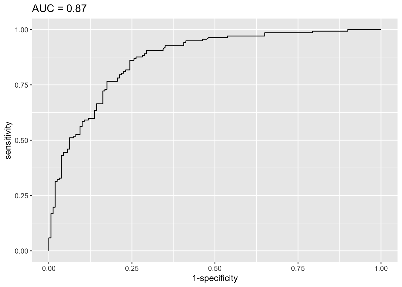
These two quality metrics can be interpreted as follows:
- in the plot, the closer the ROC curve is to the upper left-hand corner, the better the model, and
- the closer the AUC is to 1, the better the model.
Based on the ROC curve and the AUC, we can say that this model is good to very good. This means that the model is appropriate for these data, and that it can be useful to predict whether or not a patient will develop a heart disease!
Reporting results
As we have seen before, odds ratios are useful when reporting results of binary logistic regressions.
Computing these odds ratios together with the confidence intervals is not particularly difficult. However, presenting them in a table for a publication or a report can quickly become time consuming, in particular if you have many models and many independent variables.
Luckily, there are two packages which saved me a lot of time and which I use almost every time I need to report results of a logistic regression.
The first package, called {gtsummary} is useful to report results of one regression at a time. The second one is the {finalfit} package.1 This packages is more appropriate if you need to report results of several regressions at a time.
{gtsummary} package
Here is an example with one of the models built previously:
# load package
library(gtsummary)

# print table of results
tbl_regression(m5_final, exponentiate = TRUE)| Characteristic | OR1 | 95% CI1 | p-value |
|---|---|---|---|
| age | 0.74 | 0.55, 0.96 | 0.031 |
| sex | |||
| female | — | — | |
| male | 5.50 | 2.82, 11.2 | <0.001 |
| chest_pain | |||
| typical angina | — | — | |
| atypical angina | 0.99 | 0.27, 3.65 | >0.9 |
| non-anginal pain | 0.94 | 0.30, 3.07 | >0.9 |
| asymptomatic | 7.19 | 2.44, 22.8 | <0.001 |
| max_heartrate | 0.85 | 0.76, 0.94 | 0.003 |
| age * max_heartrate | 1.00 | 1.00, 1.00 | 0.013 |
| 1 OR = Odds Ratio, CI = Confidence Interval | |||
What I like with this package is its ease of use, and the fact that all results are nicely formatted in a table. This is a very good starting point when I need to create a table for a publication or a report, for one regression at a time.
The second package becomes interesting when you need to report results for several models at once.
{finalfit} package
The {finalfit} package allows to report odds ratios, their confidence intervals and the \(p\)-values in a very efficient way. Moreover, it is quite easy to do so for many regressions at the same time.
Let me present the package by reporting results of:
- all univariable binary logistic regressions that are possible with the variables available in the data frame,
- a multivariable binary logistic regression that includes all variables available in the data frame, and
- a multivariable binary logistic regression that includes only some of the variables present in the data frame.
We start with all the possible univariable binary logistic regressions:
# load packages
library(tidyverse)
library(gt)
library(finalfit)

# set dependent and independent variables
dependent <- "heart_disease"
independent <- c("age", "sex", "chest_pain", "max_heartrate")

# save results of univariable logistic regressions
glmuni <- dat |>
  glmuni(dependent, independent) |>
  fit2df(
    explanatory_name = "Variables",
    estimate_name = "Crude OR",
    estimate_suffix = " (95% CI)"
  )

# print results
glmuni |>
gt()| Variables | Crude OR (95% CI) |
|---|---|
| age | 1.05 (1.03-1.08, p<0.001) |
| sexmale | 3.57 (2.12-6.18, p<0.001) |
| chest_painatypical angina | 0.51 (0.16-1.66, p=0.255) |
| chest_painnon-anginal pain | 0.63 (0.23-1.86, p=0.384) |
| chest_painasymptomatic | 6.04 (2.39-16.76, p<0.001) |
| max_heartrate | 0.96 (0.94-0.97, p<0.001) |
A few remarks regarding this code:
glmuni()is used because we want to run univariable GLM.explanatory_name = "Variables"is used to rename the first column (by default it is “explanatory”).estimate_name = "Crude OR"is used to rename the second column and inform the reader that we are in the univariable case. In the univariable case, OR are often called crude OR because they are not adjusted for the effects of the other independent variables.estimate_suffix = " (95% CI)"is used to specify that it is the 95% confidence intervals which are inside the parentheses.- The
gt()layer at the end of the code is not compulsory. It is just to make the output appears in a nice table instead of the usual format of R outputs. See more information about the{gt}package in its documentation.
Here is how to report results of a multivariable binary logistic regression which includes all variables:
# save results of full model
glmmulti_full <- dat |>
  glmmulti(dependent, independent) |>
  fit2df(
    explanatory_name = "Variables",
    estimate_name = "Adjusted OR - full model",
  )

# print results
glmmulti_full |>
gt()| Variables | Adjusted OR - full model |
|---|---|
| age | 1.04 (1.01-1.08, p=0.024) |
| sexmale | 5.40 (2.78-10.97, p<0.001) |
| chest_painatypical angina | 0.89 (0.25-3.19, p=0.851) |
| chest_painnon-anginal pain | 0.88 (0.29-2.81, p=0.828) |
| chest_painasymptomatic | 7.13 (2.51-22.03, p<0.001) |
| max_heartrate | 0.97 (0.95-0.99, p<0.001) |
A few remarks regarding this code:
glmmulti()is used because we want to run multivariable GLM.estimate_name = "Adjusted OR - full model"is used to remind the reader that we are in the multivariable case with all variables included. In the multivariable case, OR are often called adjusted OR because they are adjusted for the effects of the other independent variables.
Here is how to report results of a multivariable binary logistic regression which includes only a selection of variables:
# select the variables to be included in the final model
independent_final <- c("age", "sex", "chest_pain")

# save results of final model
glmmulti_final <- dat |>
  glmmulti(dependent, independent_final) |>
  fit2df(
    explanatory_name = "Variables",
    estimate_name = "Adjusted OR - final model",
    estimate_suffix = " (95% CI)"
  )

# print results
glmmulti_final |>
gt()| Variables | Adjusted OR - final model (95% CI) |
|---|---|
| age | 1.07 (1.03-1.11, p<0.001) |
| sexmale | 5.52 (2.88-11.07, p<0.001) |
| chest_painatypical angina | 0.82 (0.24-2.82, p=0.743) |
| chest_painnon-anginal pain | 0.93 (0.32-2.90, p=0.903) |
| chest_painasymptomatic | 9.48 (3.47-28.53, p<0.001) |
Note that you have to manually select the variables (the package will not choose for you unfortunately). The selection could be done preliminary thanks to a stepwise procedure for example.
Now the most interesting part of this package:
- we can combine all these results together,
- in addition to some descriptive statistics for each level of the dependent variable!
Here are all results combined together and displayed in a table:
# save descriptive statistics
summary <- dat |>
  summary_factorlist(dependent, independent, fit_id = TRUE)

# save results of regressions
output <- summary |>
  finalfit_merge(glmuni) |>
  finalfit_merge(glmmulti_full) |>
  finalfit_merge(glmmulti_final)

# print all results
output |>
  dplyr::select(-fit_id, -index) |>
  dplyr::rename(
    Variables = label,
    " " = levels
  ) |>
gt()| Variables | no disease | disease | Crude OR (95% CI) | Adjusted OR - full model | Adjusted OR - final model (95% CI) | |
|---|---|---|---|---|---|---|
| age | Mean (SD) | 52.6 (9.6) | 56.8 (7.9) | 1.05 (1.03-1.08, p<0.001) | 1.04 (1.01-1.08, p=0.024) | 1.07 (1.03-1.11, p<0.001) |
| sex | female | 71 (44.4) | 25 (18.2) | - | - | - |
| male | 89 (55.6) | 112 (81.8) | 3.57 (2.12-6.18, p<0.001) | 5.40 (2.78-10.97, p<0.001) | 5.52 (2.88-11.07, p<0.001) | |
| chest_pain | typical angina | 16 (10.0) | 7 (5.1) | - | - | - |
| atypical angina | 40 (25.0) | 9 (6.6) | 0.51 (0.16-1.66, p=0.255) | 0.89 (0.25-3.19, p=0.851) | 0.82 (0.24-2.82, p=0.743) | |
| non-anginal pain | 65 (40.6) | 18 (13.1) | 0.63 (0.23-1.86, p=0.384) | 0.88 (0.29-2.81, p=0.828) | 0.93 (0.32-2.90, p=0.903) | |
| asymptomatic | 39 (24.4) | 103 (75.2) | 6.04 (2.39-16.76, p<0.001) | 7.13 (2.51-22.03, p<0.001) | 9.48 (3.47-28.53, p<0.001) | |
| max_heartrate | Mean (SD) | 158.6 (19.0) | 139.1 (22.7) | 0.96 (0.94-0.97, p<0.001) | 0.97 (0.95-0.99, p<0.001) | - |
A few remarks regarding this code:
summary_factorlist(dependent, independent, fit_id = TRUE)is used to compute the descriptive statistics by group of the dependent variable.finalfit_merge()is used to merge results together.dplyr::select(-fit_id, -index)is used to remove unnecessary columns.dplyr::rename(Variables = label, " " = levels)is used to renames some columns.
And finally, a few remarks regarding the resulting table:
- The first column gives the name of the variables.
- The second column specifies:
- for qualitative variables: the levels
- for quantitative variables: that it is the mean and the standard deviation (SD) which will be computed in the next two columns
- The third and fourth columns give the descriptive statistics for each level of the dependent variable:
- for qualitative variables: the number of cases, and in parentheses the frequencies by column
- for quantitative variables: the mean, and in parentheses the standard deviation
- The last three columns give the OR, and in parentheses the 95% CI of the OR and the \(p\)-value (for the univariable and the two multivariable models, respectively).
For your convenience, here is the full code so you can copy paste it easily in case you want to reproduce the process:
# load packages
library(tidyverse)
library(gt)
library(finalfit)

# set variables
dependent <- "heart_disease"
independent <- c("age", "sex", "chest_pain", "max_heartrate")
independent_final <- c("age", "sex", "chest_pain")

# save descriptive statistics
summary <- dat |>
  summary_factorlist(dependent, independent, fit_id = TRUE)

# save results of univariable logistic regressions
glmuni <- dat |>
  glmuni(dependent, independent) |>
  fit2df(
    explanatory_name = "Variables",
    estimate_name = "Crude OR",
    estimate_suffix = " (95% CI)"
  )

# save results of full model
glmmulti_full <- dat |>
  glmmulti(dependent, independent) |>
  fit2df(
    explanatory_name = "Variables",
    estimate_name = "Adjusted OR - full model",
  )

# save results of final model
glmmulti_final <- dat |>
  glmmulti(dependent, independent_final) |>
  fit2df(
    explanatory_name = "Variables",
    estimate_name = "Adjusted OR - final model",
    estimate_suffix = " (95% CI)"
  )

# save merged results
output <- summary |>
  finalfit_merge(glmuni) |>
  finalfit_merge(glmmulti_full) |>
  finalfit_merge(glmmulti_final)

# print all results
output |>
  dplyr::select(-fit_id, -index) |>
  dplyr::rename(
    Variables = label,
    " " = levels
  ) |>
  gt()
Last but not least, the or_plot() function, also available from the {finalfit} package, is useful to visualize all odds ratio and their 95% confidence intervals:
dat |> or_plot(dependent, independent,
  table_text_size = 3.5 # reduce text size
)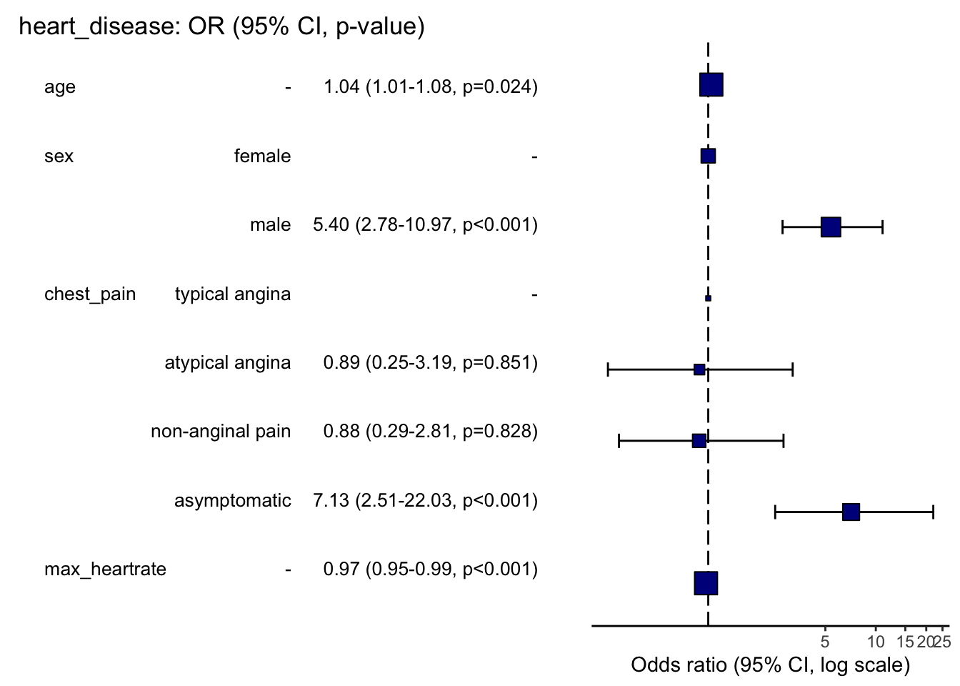
Here is how to read this plot:
- The squares represent the OR, and the whiskers their 95% CI.
- When the 95% CI crosses the vertical dashed line, it means that the OR is not significantly different from 1 (at the 5% significance level). In these cases, we cannot reject the hypothesis of no association with the dependent variable.
- When the 95% CI does not cross the vertical dashed line, it means that the OR is significantly different from 1. In these cases:
- if the square is located to the right of the vertical dashed line, there is a positive relationship between the outcome and the independent variable (known as a risk factor), and
- if the square is located to the left of the vertical dashed line, there is a negative relationship between the outcome and the independent variable (known as a protective factor).
The plot confirms what was obtained above:
- age is a risk factor for heart disease,
- maximum heart rate achieved is a protective factor for heart disease, and
- being a male and suffering from asymptomatic chest pain are both risk factors of heart disease.
Be careful that sometimes the square is too big to see the whiskers of the 95% CI. This is the case for the variables max_heartrate and age. In these cases, it is better to check the significance of the OR thanks to their 95% CI or the \(p\)-values printed in parentheses.
Conditions of application
For results to be valid and interpretable, a binary logistic regression requires:
- the dependent variable to be binary,
- independence of the observations: no repeated measurements or matched data, otherwise generalize linear mixed effect models (GLMM) should be used,
- linearity of continuous independent variables and the log-odds outcome: take age and heart disease as an example. If heart disease is more frequent or less frequent as age rises, the model will work well. However, if children and the elderly are at high risk of having a heart disease, but those in middle years are not, then the relationship is not linear, or not monotonic, meaning that the response does not only go in one direction,
- a sufficiently large sample size (for confidence intervals and hypothesis tests to be valid), and
- no multicollinearity: independent variables should not be highly correlated with each other, otherwise coefficients and OR can become unstable.
Here is how to verify each of them:
- this is obvious; check if the dependent variable has indeed only two levels,
- this is often not tested formally, but verified through the design of the experiment,
- quantitative independent variables should have a linear relationship between their log-odds and their observed values. A visual check is sufficient, see below with age, maximum heart rate achieved and model
m3as example:
# linearity to the log-odds?
dat |>
  dplyr::select(age, max_heartrate) |>
  mutate(log_odds = predict(m3)) |>
  pivot_longer(-log_odds) |>
  ggplot(aes(log_odds, value)) +
  geom_point() +
  geom_smooth(method = "lm") +
  facet_wrap(~name)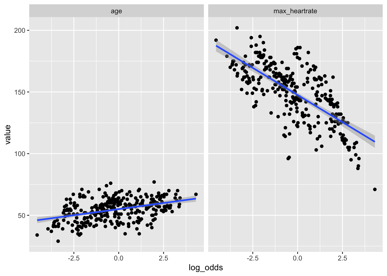
- in practice, it is recommended to have at least 10 times as many events as parameters in the model, and
- the variance inflation factors (VIF) is a well known measure of multicollinearity. It should be below 10 or 5, depending on the field of research. VIF can be computed with the
vif()function, available in the{car}package:
# load package
library(car)

# compute VIF for model m3
vif(m3)
## GVIF Df GVIF^(1/(2*Df))
## age 1.205246 1 1.097837
## sex 1.155071 1 1.074742
## chest_pain 1.113010 3 1.018005
## max_heartrate 1.143125 1 1.069170Conclusion
Thanks for reading.
In this relatively long and detailed post, we covered several important points about binary logistic regression. First, when to use such models and what is the difference with linear models, how to implement it in R, and how to interpret and report results. We ended by discussing about model selection, how to judge the quality of fit of a logistic regression, and its underlying assumptions.
I now hope that (univariable and multivariable) binary logistic regressions in R no longer hold any secrets for you.
As always, if you have a question or a suggestion related to the topic covered in this article, please add it as a comment so other readers can benefit from the discussion.
Thanks to Claire from DellaData.fr for introducing me to this package.↩︎
Liked this post?
- Get updates every time a new article is published (no spam and unsubscribe anytime)
- Support the blog
- Share on:


