
What is the probability that two persons have the same initials?

Introduction
Last week, I joined a team to work on a collaborative project. The team was already established for a few months, with several scientists working together on the project. For simplicity, they used to sign documents, mention colleagues in emails, etc. with their initials (the first letter of their first name followed by the first letter of their last name).
A couple of days after joining the project, when I needed to sign my first document with my initials, we realized that another person in the team had the exact same initials than me.
This was not really an issue, as we decided that I would write my initials backward, that is, “SA” instead of “AS”, and the other person would keep signing with “AS” as usual.
It could have stopped here. However, the idea to write a post about this rather trivial anecdote came to me when the team leader claimed, in the middle of a meeting: “That’s very unfortunate that you two have the same initials! What are the chances of this happening to us?!”.
We spent a couple of minutes trying to estimate this probability, which in the end were mostly based on our intuitions rather than on a formal calculation. This piqued my curiosity.
Given that the project we are working on requires the use of simulations, I decided to focus on answering this question via simulations in R. That being said, as for most simulations, it is a good practice to verify these results. This is done using probability theory. This comparison will allow to assess the truthfulness of results obtained through simulations.
Furthermore, I thought that it would be a nice way to illustrate methods not often presented in my posts: for loops, replications and writing functions in R.
How likely is it?
Before answering the question raised by the team leader, there are three things to note:
- Although the team leader was curious to know the probability that exactly two persons have the same initials, we are actually more interested in the probability that at least two persons have the same initials (as the problem also occurs if more than two persons within a team have the same initials).
- The team consists of 8 people.
- We restrict ourselves to two-letters initials (the first letter being the first letter of the first name, the second letter being the first letter of the last name). This means that middle names are not taken into account, and only the first letter is considered for compound names.
In this post, we will show how to compute this probability:
- in our context, that is, for a team of 8 persons, and
- for completeness, for teams of all sizes from 2 to 100 persons.
As stated in the introduction, we will compute these probabilities first through simulations and then through probability theory.
For our team
We start by creating a vector of size 8, corresponding to the initials of a team of 8 persons randomly sampled among all 26 letters of the Latin alphabet:
# number of persons
n_persons <- 8

# create vector of initials
initials <- replicate(
  n = n_persons, # number of replications
  paste0(sample(LETTERS, size = 1), sample(LETTERS, size = 1)) # sample letters
)

# display initials
initials
## [1] "UJ" "MN" "XD" "CY" "BB" "ZB" "CU" "HQ"# are there duplicates?
any(duplicated(initials))## [1] FALSEAs we can see, everyone has different initials in this simulated team of 8 persons, but this will not always be the case.
To estimate, via simulations, how likely is that at least two persons have the same initials among the team, we need to replicate this vector of 8 sampled initials a large number of times (say 1,000 replications):1
# number of replications
reps <- 1000

# create and save replications
dat <- replicate(
  n = reps, # number of replications
  replicate(n_persons, paste0(sample(LETTERS, size = 1), sample(LETTERS, size = 1)))
)

# dimensions
dim(dat)
## [1] 8 1000# display first 4 simulated teams
dat[, 1:4]## [,1] [,2] [,3] [,4]
## [1,] "VA" "BU" "LU" "PT"
## [2,] "JG" "SM" "HM" "OL"
## [3,] "BY" "NA" "VJ" "OT"
## [4,] "RT" "CM" "WT" "YT"
## [5,] "PS" "CT" "NB" "QJ"
## [6,] "MG" "KR" "SV" "US"
## [7,] "PL" "SN" "PN" "XW"
## [8,] "NJ" "BR" "DD" "ZC"The result is a matrix of 8 rows and 1000 columns, where:
- each rows corresponds to the sampled initials of a person, and
- each column corresponds to one simulated team of 8 people.
For better readability, we rename:
- the row names as
M1toM8, corresponding to persons 1 to 8, and - the column names as
T1toT1000, corresponding to teams 1 to 1000.
# rename rows
rownames(dat) <- paste0("M", 1:n_persons)
# rename columns
colnames(dat) <- paste0("T", 1:reps)
# display first 4 simulated teams
dat[, 1:4]
## T1 T2 T3 T4
## M1 "VA" "BU" "LU" "PT"
## M2 "JG" "SM" "HM" "OL"
## M3 "BY" "NA" "VJ" "OT"
## M4 "RT" "CM" "WT" "YT"
## M5 "PS" "CT" "NB" "QJ"
## M6 "MG" "KR" "SV" "US"
## M7 "PL" "SN" "PN" "XW"
## M8 "NJ" "BR" "DD" "ZC"We now need to compute, among the 1000 teams simulated, how many of them have at least two persons with the same initials:
# transform to data frame
dat <- as.data.frame(dat)

# save which teams have duplicates
duplicates <- rep(NA, reps) # create empty vector
for (i in 1:reps) { # for loop over i from 1 to 1,000
  duplicates[i] <- any(duplicated(dat[, i])) # save results TRUE/FALSE in duplicates vector
}

# count how many teams have duplicates
sum(duplicates)
## [1] 41Here, for each column of our data frame dat (from the first to the 1000th column), we ask whether there are duplicates or not. This is done repeatedly over all columns thanks to a for loop. For each column, the result is TRUE if there are duplicates, otherwise it is FALSE. The result of each iteration is saved in the duplicates vector. As TRUE = 1 and FALSE = 0 in R, we can then count how many columns (and thus teams) have duplicates by summing the number of TRUE in the duplicates vector.
As we can see from the output above, among the 1000 simulated teams, 41 of them have duplicates, that is, 41 of them have at least two persons with the same initials.
Therefore, based on the simulations, we can expect the probability that at least two persons with the same initials in a team of 8 persons to be close to 4.1%.
This is a good starting point. Notice, however, that I wrote close to 4.1% because this probability will vary each time it is computed via simulations.
For instance, if we repeat the exact same process a second time:
# create and save replications
dat <- replicate(
  n = reps, # number of replications
  replicate(n_persons, paste0(sample(LETTERS, size = 1), sample(LETTERS, size = 1)))
)

# transform to data frame
dat <- as.data.frame(dat)

# save which teams have duplicates
duplicates <- rep(NA, reps) # create empty vector
for (i in 1:reps) { # for loop over i from 1 to 1,000
  duplicates[i] <- any(duplicated(dat[, i])) # save results in the duplicates vector (as TRUE/FALSE)
}

# count how many teams have duplicates
sum(duplicates)
## [1] 44We now find a probability of 4.4%. This is not an error, but it is due to randomness when sampling initials.
Luckily, we can make the computation of this probability more robust thanks to replications. Intuitively, it works as follows. We repeat the same computation multiple times, giving us a range of possible probabilities. This allows us to assess the uncertainty of our result, and understand how the probability might vary due to taking different random samples of initials.
So the goal is to compute our probability multiple times (say 100 times), and see its distribution.
To repeat the same computation multiple times, it is best to write a function in order to avoid copy pasting the same code over and over. So we first write a function (called initials) which computes the probability that at least two persons share the same initials among a team of \(n\) people:
initials <- function(n_persons, reps = 1000) {
  # simulate data
  dat <- as.data.frame(replicate(
    reps,
    replicate(n_persons, paste0(sample(LETTERS, size = 1), sample(LETTERS, size = 1)))
  ))

  # save which teams have duplicates
  duplicates <- rep(NA, reps)
  for (i in 1:reps) {
    duplicates[i] <- any(duplicated(dat[, i]))
  }

  # proportion of teams with duplicates
  return(mean(duplicates))
}
A function in R requires to include:
- the parameters inside
(), and - the computation inside
{}.
We can then use our function to compute the probability that at least two persons share the same initials among a team of 8 people. And we combine it with the replicate() function to compute this probability 100 times.
# compute and save probabilities
probs <- replicate(100, initials(n_persons = 8))

# display probabilities
probs
## [1] 0.032 0.037 0.040 0.043 0.033 0.042 0.039 0.047 0.045 0.038 0.052 0.042
## [13] 0.042 0.040 0.023 0.044 0.041 0.039 0.036 0.048 0.041 0.037 0.027 0.030
## [25] 0.052 0.038 0.043 0.035 0.038 0.045 0.047 0.044 0.030 0.036 0.036 0.048
## [37] 0.038 0.045 0.044 0.034 0.031 0.043 0.045 0.034 0.049 0.047 0.051 0.036
## [49] 0.051 0.040 0.043 0.044 0.038 0.049 0.043 0.050 0.035 0.043 0.048 0.038
## [61] 0.041 0.044 0.039 0.045 0.033 0.057 0.036 0.043 0.041 0.041 0.041 0.041
## [73] 0.038 0.044 0.031 0.034 0.049 0.041 0.040 0.034 0.032 0.036 0.049 0.047
## [85] 0.048 0.038 0.038 0.037 0.036 0.037 0.043 0.040 0.026 0.049 0.046 0.044
## [97] 0.048 0.038 0.026 0.029Finally, we visualize the distribution of these 100 probabilities thanks to a histogram and a boxplot (with the {ggplot2} package):
# visualize distribution of the computed probabilities
# build and save plots
library(ggplot2)

p1 <- ggplot(mapping = aes(x = probs)) +
  geom_histogram(color = "black", fill = "steelblue", bins = 8) +
  labs(
    x = "Probabilities",
    y = "Frequencies"
  ) +
  scale_x_continuous(labels = scales::percent) # format x-axis in %

p2 <- ggplot(mapping = aes(x = probs)) +
  geom_boxplot(color = "black", fill = "steelblue") +
  labs(x = "Probabilities") +
  theme(
    axis.text.y = element_blank(),
    axis.ticks.y = element_blank()
  ) +
  scale_x_continuous(labels = scales::percent) # format x-axis in %

# combine plots
library(patchwork)

p1 + p2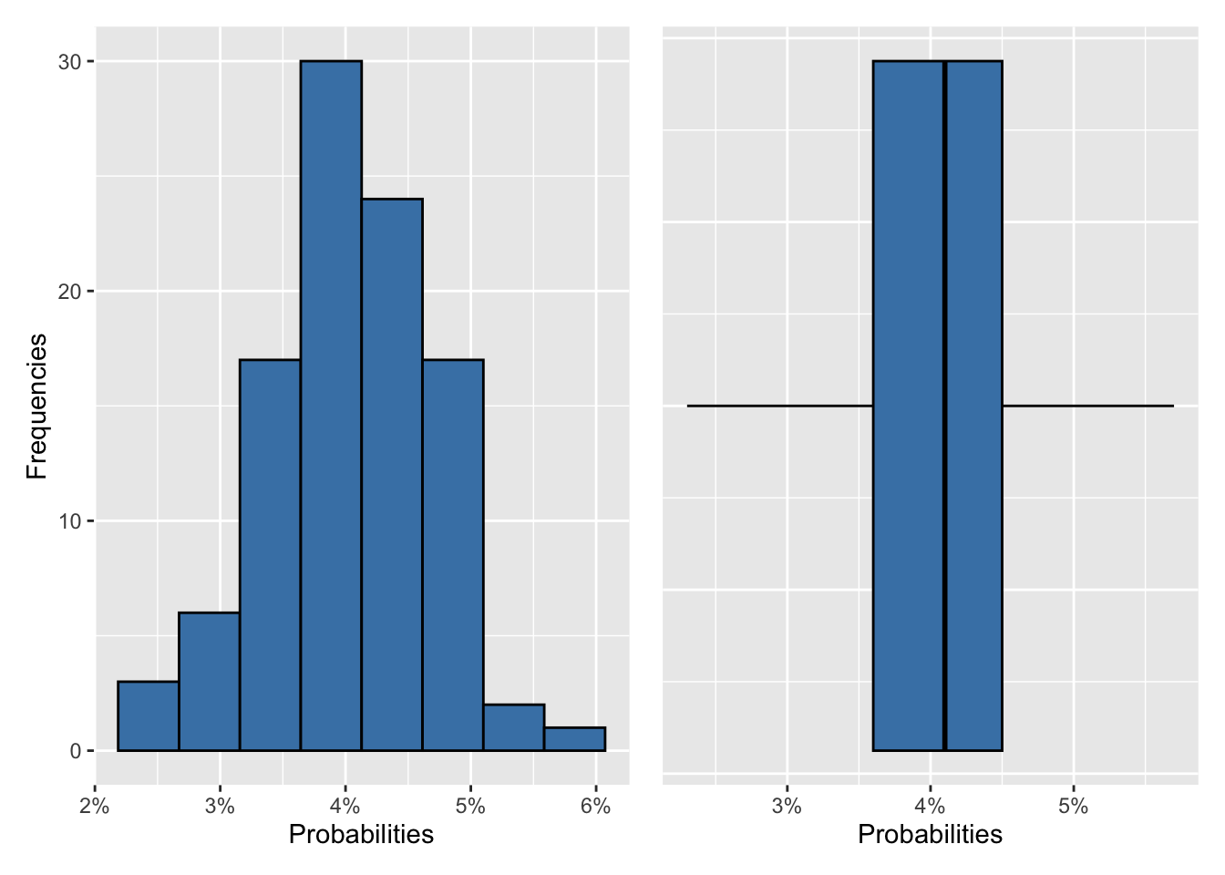
These two plots show that the probability that at least two persons share the same initials among a team of 8 people is most likely between 3.5% and 4.5%.
For the record, during the meeting at the root of all this thinking, most of us thought that it was much less likely. Indeed, I believe we were tempted to compute the probability that someone who joins the team has “AS” as initials. This is indeed much less likely, as the probability is only \(\frac{1}{26} \times \frac{1}{26} \simeq 0.15\%\).
However, this does not take into account the fact:
- that the newcomer can have the same initials as any other person, and
- that it is not only the newcomer who can have the same initials as another person (2 people already working in the team when the newcomer arrives could have the same initials as well).
If you are puzzled by this finding, I recommend reading about the birthday’s paradox. The birthday’s paradox states that the probability of two people sharing the same birthday becomes surprisingly high with a relatively small group of individuals. In practice, in a group of just 23 people, there is a greater than 50% chance that at least two individuals share the same birthday, illustrating our counterintuitive intuitions about the likelihood of such coincidences. This phenomenon arises due to the multitude of possible birthday pairs within the group, similar to the multitude of possible pairs if initials within a team.
For teams of different sizes
We are now interested in computing this probability not just for a team of 8 persons, but for teams of different sizes. We can do this with the help of our function defined earlier.
For the illustration, let’s compute the probability that at least two persons have the same initials, for teams of 2 and up to 100 persons:
# set lower and upper bounds of number of persons
min_persons <- 2
max_persons <- 100

# create empty vector of probabilities
probs <- rep(NA, length(min_persons:max_persons))

# compute and save probabilities for teams of size 2 to 100
for (i in min_persons:max_persons) {
  probs[i] <- initials(n_persons = i)
}

# display probabilities
probs
## [1] NA 0.001 0.005 0.013 0.012 0.019 0.036 0.040 0.047 0.057 0.074 0.083
## [13] 0.103 0.128 0.158 0.166 0.178 0.215 0.232 0.260 0.275 0.296 0.300 0.329
## [25] 0.357 0.392 0.405 0.405 0.439 0.478 0.495 0.536 0.535 0.563 0.578 0.599
## [37] 0.653 0.656 0.686 0.693 0.715 0.711 0.767 0.760 0.786 0.784 0.814 0.817
## [49] 0.825 0.826 0.842 0.845 0.867 0.893 0.901 0.920 0.919 0.911 0.917 0.942
## [61] 0.950 0.951 0.946 0.947 0.969 0.959 0.965 0.964 0.977 0.984 0.977 0.977
## [73] 0.985 0.978 0.986 0.981 0.989 0.991 0.989 0.988 0.992 0.993 0.994 0.996
## [85] 0.997 0.995 0.994 0.999 0.999 0.999 1.000 0.999 0.997 1.000 0.999 0.999
## [97] 0.999 1.000 1.000 0.999We are left with storing these probabilities together with the number of persons in the team in a data frame:
# create data frame with saved probabilities and number of persons
dat_plot_sim <- data.frame(
  n_persons = (min_persons - 1):max_persons,
  prob = probs
)

# display first 6 rows
head(dat_plot_sim)
## n_persons prob
## 1 1 NA
## 2 2 0.001
## 3 3 0.005
## 4 4 0.013
## 5 5 0.012
## 6 6 0.019Of course, two people having the same initials in a team of 1 (if we can call this a team…) is impossible.
An event which is impossible has a probability equal to 0. We thus impute this probability in our data frame, in the first row:
# set proba = 0 when n_person = 1
dat_plot_sim[1, 2] <- 0

# display first 6 rows
head(dat_plot_sim)
## n_persons prob
## 1 1 0.000
## 2 2 0.001
## 3 3 0.005
## 4 4 0.013
## 5 5 0.012
## 6 6 0.019Finally, we visualize these probabilities in function of the number of persons in the team:
# visualize probabilities
ggplot(dat_plot_sim) +
  aes(x = n_persons, y = probs) +
  geom_line(linewidth = 1) +
  labs(
    x = "# of persons in the team",
    y = "Probability",
    title = "What is the probability that at least 2 persons have the same initials?"
  ) +
  scale_y_continuous(labels = scales::percent) # format y-axis in %
From the plot above, we see that the probability that at least two persons have the same initials reaches 50% when the team exceeds around 30 people.
Moreover, notice that this probability becomes close to 100% when the team reaches around 75 people.
Verification
For the sake of completeness, we now compare results obtained through simulations with results obtained from probability theory.2
We first define the function that will be used to compare results found above:
# define function
have_same <- function(s, n) {
  sample_space <- s
  probability <- 1
  for (i in 0:(n - 1)) {
    probability <- probability * (sample_space - i) / sample_space
  }
  1 - probability
}
For our team
# number of possible two-letter initials
n_initials <- 26^2

# apply function
have_same(n_initials, n_persons)
## [1] 0.0407218The probability that at least two persons have the same initials in a team of 8 is 4.07%. This is close to the probability found with simulations, and within the range of 3.5%–4.5%.
For teams of different sizes
We now compute the probability for teams between 1 and 100 persons:
# compute and save probabilities for teams between 1 and 100 persons
probs <- vector(length = max_persons)
for (i in 1:max_persons) {
  probs[i] <- have_same(n_initials, i)
}

# create data frame with saved probabilities and number of persons
dat_plot_theory <- data.frame(
  n_persons = (min_persons - 1):max_persons,
  prob = probs
)

# display first 6 rows
head(dat_plot_theory)
## n_persons prob
## 1 1 0.000000000
## 2 2 0.001479290
## 3 3 0.004433493
## 4 4 0.008851688
## 5 5 0.014716471
## 6 6 0.022004071Finally, we visualize these probabilities in function of the number of persons in the team:
# visualize probabilities
ggplot(dat_plot_theory) +
  aes(x = n_persons, y = probs) +
  geom_line(linewidth = 1) +
  labs(
    x = "# of persons in the team",
    y = "Probability",
    title = "What is the probability that at least 2 persons have the same initials?"
  ) +
  scale_y_continuous(labels = scales::percent) # format y-axis in %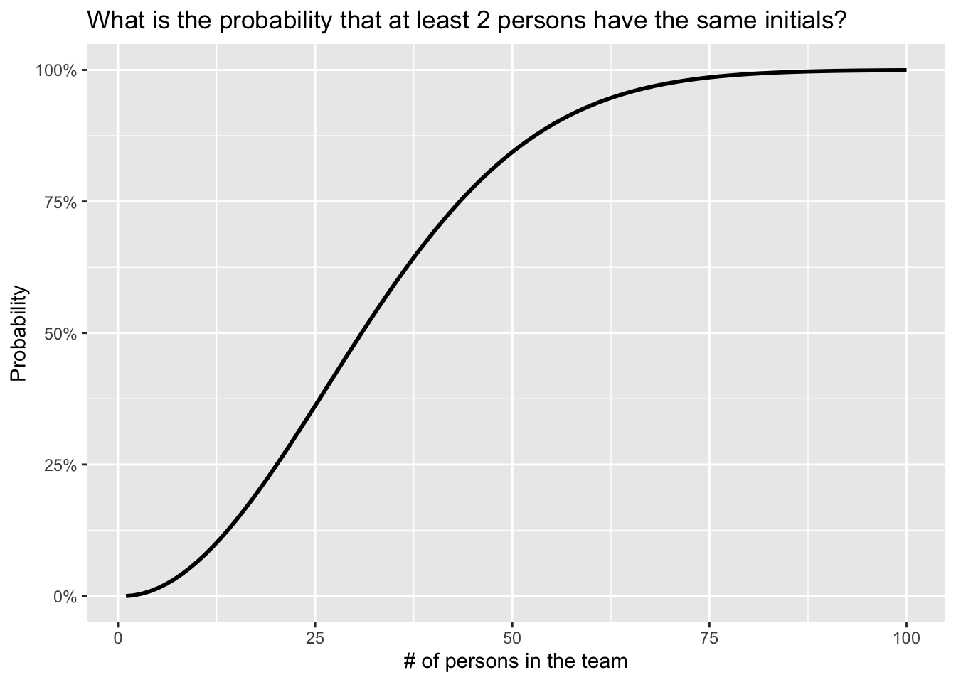
For an easier comparison, we plot probabilities found thanks to simulations and thanks to probability theory on the same plot:
# combine the two data frames into one and add the method as variable
dat_plot_sim$Method <- "Simulations"
dat_plot_theory$Method <- "Theory"
dat_plot_all <- rbind(dat_plot_sim, dat_plot_theory)

# visualize probabilities on same plot
ggplot(dat_plot_all) +
  aes(x = n_persons, y = prob, color = Method) +
  geom_line(linewidth = 1) +
  labs(
    x = "# of persons in the team",
    y = "Probability",
    title = "What is the probability that at least 2 persons have the same initials?"
  ) +
  scale_y_continuous(labels = scales::percent) # format y-axis in %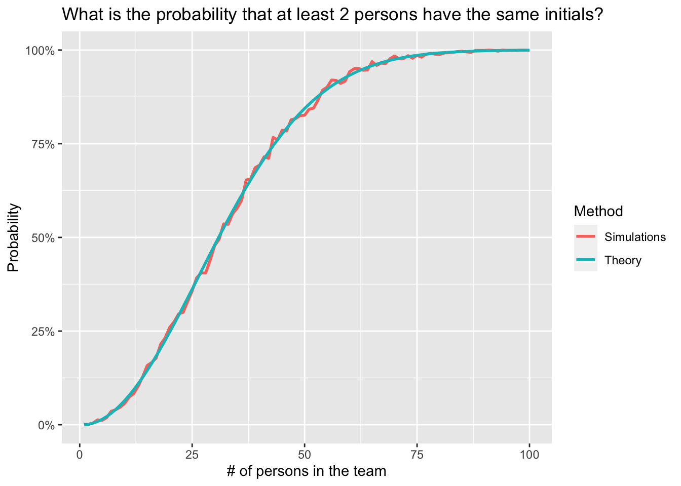
The plot above shows that results using probability theory are relatively similar to results obtained through simulations, indicating that the simulations are trustworthy.
Conclusion
The initial question, raised during a meeting, was “What is the probability that, among our team consisting of 8 persons, two have the same initials?”.
In this post, we first showed how to compute this probability through simulations in R. Secondly, we verified the veracity of the simulations thanks to probability theory. Furthermore, we illustrated how for loops, replications and writing a function can be used in R to answer a probability problem.
As a side note, it is important to keep in mind that in this post, we assumed the following:
- All letters of the alphabet had the same probability of occurring, meaning that all pairs of initials were equally probable. This is probably not the case in reality, as a first and last name starting both with X is not as probable as a first and last name starting respectively with M and K. This bias could be limited by specifying different weights when sampling initials.
- We restricted ourselves to two-letters initials. Therefore, for compound first or last names, only the first letter is considered. Middle names are also not taken into account.
Last but not least, note that you will find slightly different results than mine, even if you use the exact same code. This is due to randomness. To replicate results as shown in this post, use set.seed(6).
Thanks for reading.
As always, if you have a question or a suggestion related to the topic covered in this article, please add it as a comment so other readers can benefit from the discussion.
Liked this post?
- Get updates every time a new article is published (no spam and unsubscribe anytime)
- Support the blog
- Share on:


