The complete guide to clustering analysis: k-means and hierarchical clustering by hand and in R
- What is clustering analysis?
- k-means clustering
- Hierarchical clustering
- k-means versus hierarchical clustering
- What’s next?
- Conclusion
- References

Note that this article is inspired from the lecture notes of Prof. Johan Segers and my personal notes as teaching assistant for his course entitled “Multivariate statistical analysis” given at UCLouvain.
What is clustering analysis?
Clustering analysis is a form of exploratory data analysis in which observations are divided into different groups that share common characteristics.
The purpose of cluster analysis (also known as classification) is to construct groups (or classes or clusters) while ensuring the following property: within a group the observations must be as similar as possible (intracluster similarity), while observations belonging to different groups must be as different as possible (intercluster similarity).
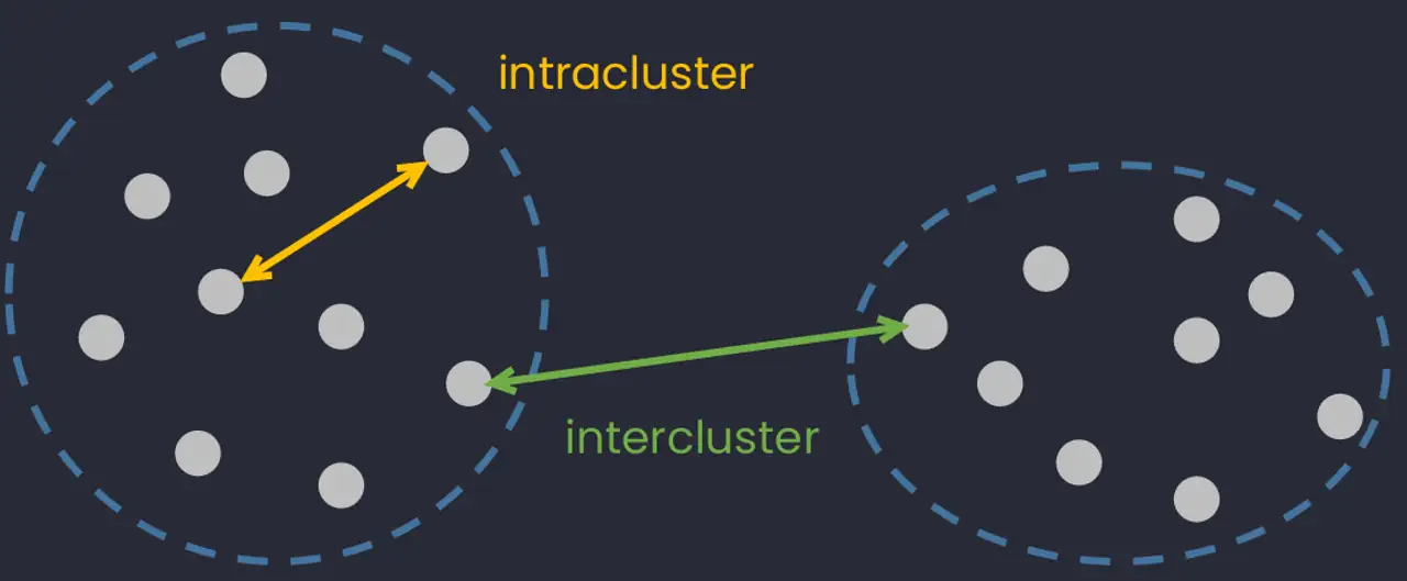
The two most common types of classification are:
- k-means clustering
- Hierarchical clustering
The first is generally used when the number of classes is fixed in advance, while the second is generally used for an unknown number of classes and helps to determine this optimal number. For this reason, k-means is considered as a supervised technique, while hierarchical clustering is considered as an unsupervised technique because the estimation of the number of clusters is part of the algorithm. See more clustering methods in this article.
Both methods are illustrated below through applications by hand and in R. Note that for hierarchical clustering, only the ascending classification is presented in this article.
Clustering algorithms use the distance in order to separate observations into different groups. Therefore, before diving into the presentation of the two classification methods, a reminder exercise on how to compute distances between points is presented.
Application 1: Computing distances
Let a data set containing the points \(\boldsymbol{a} = (0, 0)'\), \(\boldsymbol{b} = (1, 0)'\) and \(\boldsymbol{c} = (5, 5)'\). Compute the matrix of Euclidean distances between the points by hand and in R.
Solution
The points are as follows:
# We create the points in R
a <- c(0, 0)
b <- c(1, 0)
c <- c(5, 5)

X <- rbind(a, b, c) # a, b and c are combined per row
colnames(X) <- c("x", "y") # rename columns

X # display the points
## x y
## a 0 0
## b 1 0
## c 5 5By the Pythagorean theorem, we will remember that the distance between 2 points \((x_a, y_a)\) and \((x_b, y_b)\) in \(\mathbb{R}^2\) is given by \(\sqrt{(x_a - x_b)^2 + (y_a - y_b)^2}\). So for instance, for the distance between the points \(\boldsymbol{b} = (1, 0)'\) and \(\boldsymbol{c} = (5, 5)'\) presented in the statement above, we have:
\[\begin{equation} \begin{split} d(b, c) &= \sqrt{(x_b - x_c)^2 + (y_b - y_c)^2} \\ &= \sqrt{(1-5)^2 + (0-5)^2}\\ &= 6.403124 \end{split} \end{equation}\]
We can proceed similarly for all pairs of points to find the distance matrix by hand. In R, the dist() function allows you to find the distance of points in a matrix or dataframe in a very simple way:
# The distance is found using the dist() function:
distance <- dist(X, method = "euclidean")
distance # display the distance matrix
## a b
## b 1.000000
## c 7.071068 6.403124Note that the argument method = "euclidean" is not mandatory because the Euclidean method is the default one.
The distance matrix resulting from the dist() function gives the distance between the different points. The Euclidean distance between the points \(\boldsymbol{b}\) and \(\boldsymbol{c}\) is 6.403124, which corresponds to what we found above via the Pythagorean formula.
Note: If two variables do not have the same units, one may have more weight in the calculation of the Euclidean distance than the other. In that case, it is preferable to scale the data. Scaling data allows to obtain variables independent of their unit, and this can be done with the scale() function.
Now that the distance has been presented, let’s see how to perform clustering analysis with the k-means algorithm.
k-means clustering
The first form of classification is the method called k-means clustering or the mobile center algorithm. As a reminder, this method aims at partitioning \(n\) observations into \(k\) clusters in which each observation belongs to the cluster with the closest average, serving as a prototype of the cluster.
We do not go too much into details about the mathematics. Instead, we focus on how to apply it in R and by hand.
Application 2: k-means clustering
Data
For this exercise, the Eurojobs.csv database available here is used.
This database contains the percentage of the population employed in different industries in 26 European countries in 1979. It contains 10 variables:
Country- the name of the country (identifier)Agr- % of workforce employed in agricultureMin- % in miningMan- % in manufacturingPS- % in power supplies industriesCon- % in constructionSI- % in service industriesFin- % in financeSPS- % in social and personal servicesTC- % in transportation and communications
We first import the dataset. See how to import data into R if you need a reminder.
# Import data
Eurojobs <- read.csv(
  file = "https://statsandr.com/blog/data/Eurojobs.csv",
  sep = ",",
  dec = ".",
  header = TRUE
)

head(Eurojobs) # head() is used to display only the first 6 observations
## Country Agr Min Man PS Con SI Fin SPS TC
## 1 Belgium 3.3 0.9 27.6 0.9 8.2 19.1 6.2 26.6 7.2
## 2 Denmark 9.2 0.1 21.8 0.6 8.3 14.6 6.5 32.2 7.1
## 3 France 10.8 0.8 27.5 0.9 8.9 16.8 6.0 22.6 5.7
## 4 W. Germany 6.7 1.3 35.8 0.9 7.3 14.4 5.0 22.3 6.1
## 5 Ireland 23.2 1.0 20.7 1.3 7.5 16.8 2.8 20.8 6.1
## 6 Italy 15.9 0.6 27.6 0.5 10.0 18.1 1.6 20.1 5.7Note that there is a numbering before the first variable Country. For more clarity, we will replace this numbering by the country. To do this, we add the argument row.names = 1 in the import function read.csv() to specify that the first column corresponds to the row names:
Eurojobs <- read.csv(
  file = "https://statsandr.com/blog/data/Eurojobs.csv",
  sep = ",",
  dec = ".",
  header = TRUE,
  row.names = 1
)

Eurojobs # displays dataset
## Agr Min Man PS Con SI Fin SPS TC
## Belgium 3.3 0.9 27.6 0.9 8.2 19.1 6.2 26.6 7.2
## Denmark 9.2 0.1 21.8 0.6 8.3 14.6 6.5 32.2 7.1
## France 10.8 0.8 27.5 0.9 8.9 16.8 6.0 22.6 5.7
## W. Germany 6.7 1.3 35.8 0.9 7.3 14.4 5.0 22.3 6.1
## Ireland 23.2 1.0 20.7 1.3 7.5 16.8 2.8 20.8 6.1
## Italy 15.9 0.6 27.6 0.5 10.0 18.1 1.6 20.1 5.7
## Luxembourg 7.7 3.1 30.8 0.8 9.2 18.5 4.6 19.2 6.2
## Netherlands 6.3 0.1 22.5 1.0 9.9 18.0 6.8 28.5 6.8
## United Kingdom 2.7 1.4 30.2 1.4 6.9 16.9 5.7 28.3 6.4
## Austria 12.7 1.1 30.2 1.4 9.0 16.8 4.9 16.8 7.0
## Finland 13.0 0.4 25.9 1.3 7.4 14.7 5.5 24.3 7.6
## Greece 41.4 0.6 17.6 0.6 8.1 11.5 2.4 11.0 6.7
## Norway 9.0 0.5 22.4 0.8 8.6 16.9 4.7 27.6 9.4
## Portugal 27.8 0.3 24.5 0.6 8.4 13.3 2.7 16.7 5.7
## Spain 22.9 0.8 28.5 0.7 11.5 9.7 8.5 11.8 5.5
## Sweden 6.1 0.4 25.9 0.8 7.2 14.4 6.0 32.4 6.8
## Switzerland 7.7 0.2 37.8 0.8 9.5 17.5 5.3 15.4 5.7
## Turkey 66.8 0.7 7.9 0.1 2.8 5.2 1.1 11.9 3.2
## Bulgaria 23.6 1.9 32.3 0.6 7.9 8.0 0.7 18.2 6.7
## Czechoslovakia 16.5 2.9 35.5 1.2 8.7 9.2 0.9 17.9 7.0
## E. Germany 4.2 2.9 41.2 1.3 7.6 11.2 1.2 22.1 8.4
## Hungary 21.7 3.1 29.6 1.9 8.2 9.4 0.9 17.2 8.0
## Poland 31.1 2.5 25.7 0.9 8.4 7.5 0.9 16.1 6.9
## Rumania 34.7 2.1 30.1 0.6 8.7 5.9 1.3 11.7 5.0
## USSR 23.7 1.4 25.8 0.6 9.2 6.1 0.5 23.6 9.3
## Yugoslavia 48.7 1.5 16.8 1.1 4.9 6.4 11.3 5.3 4.0dim(Eurojobs) # displays the number of rows and columns## [1] 26 9We now have a “clean” dataset of 26 observations and 9 quantitative continuous variables on which we can base the classification. Note that in this case it is not necessary to standardize the data because they are all expressed in the same unit (in percentage). If this was not the case, we would have had to standardize the data via the scale() function (do not forget it otherwise your results may be completely different!).
The so-called k-means clustering is done via the kmeans() function, with the argument centers that corresponds to the number of desired clusters. In the following we apply the classification with 2 classes and then 3 classes as examples.
kmeans() with 2 groups
model <- kmeans(Eurojobs, centers = 2)

# displays the class determined by
# the model for all observations:
model$cluster
## Belgium Denmark France W. Germany Ireland
## 1 1 1 1 2
## Italy Luxembourg Netherlands United Kingdom Austria
## 1 1 1 1 1
## Finland Greece Norway Portugal Spain
## 1 2 1 2 2
## Sweden Switzerland Turkey Bulgaria Czechoslovakia
## 1 1 2 2 1
## E. Germany Hungary Poland Rumania USSR
## 1 2 2 2 2
## Yugoslavia
## 2Note that the argument centers = 2 is used to set the number of clusters, determined in advance. In this exercise the number of clusters has been determined arbitrarily.
This number of clusters should be determined according to the context and goal of your analysis (so according to your expectations or hypotheses), or based on methods explained in this section. The output model$cluster specifies the group (i.e., 1 or 2) to which each country belongs to.
The cluster for each observation can be stored directly in the dataset as a column:
Eurojobs_cluster <- data.frame(Eurojobs,
  cluster = as.factor(model$cluster)
)

head(Eurojobs_cluster)
## Agr Min Man PS Con SI Fin SPS TC cluster
## Belgium 3.3 0.9 27.6 0.9 8.2 19.1 6.2 26.6 7.2 1
## Denmark 9.2 0.1 21.8 0.6 8.3 14.6 6.5 32.2 7.1 1
## France 10.8 0.8 27.5 0.9 8.9 16.8 6.0 22.6 5.7 1
## W. Germany 6.7 1.3 35.8 0.9 7.3 14.4 5.0 22.3 6.1 1
## Ireland 23.2 1.0 20.7 1.3 7.5 16.8 2.8 20.8 6.1 2
## Italy 15.9 0.6 27.6 0.5 10.0 18.1 1.6 20.1 5.7 1Quality of a k-means partition
The quality of a k-means partition is found by calculating the percentage of the TSS “explained” by the partition using the following formula:
\[\begin{equation} \dfrac{\operatorname{BSS}}{\operatorname{TSS}} \times 100\% \end{equation}\]
where BSS and TSS stand for Between Sum of Squares and Total Sum of Squares, respectively. The higher the percentage, the better the score (and thus the quality) because it means that BSS is large and/or WSS is small.
Here is how you can check the quality of the partition in R:
# BSS and TSS are extracted from the model and stored
(BSS <- model$betweenss)
## [1] 4823.535(TSS <- model$totss)## [1] 9299.59# We calculate the quality of the partition
BSS / TSS * 100## [1] 51.86826The quality of the partition is 51.87%. This value has no real interpretation in absolute terms except that a higher quality means a higher explained percentage. However, it is more insightful when it is compared to the quality of other partitions (with the same number of clusters! see why at the end of this section) in order to determine the best partition among the ones considered.
nstart for several initial centers and better stability
Note that k-means is a non-deterministic algorithm so running it multiple times may result in different classification. This is the case because the k-means algorithm uses a random set of initial points to arrive at the final classification. Due to the fact that the initial centers are randomly chosen, the same command kmeans(Eurojobs, centers = 2) may give different results every time it is run, and thus slight differences in the quality of the partitions. The nstart argument in the kmeans() function allows to run the algorithm several times with different initial centers, in order to obtain a potentially better partition:
model2 <- kmeans(Eurojobs, centers = 2, nstart = 10)
100 * model2$betweenss / model2$totss
## [1] 54.2503Depending on the initial random choices, this new partition will be better or not compared to the first one. In our example, the partition is better as the quality increased to 54.25%.
One of the main limitation often cited regarding k-means is the stability of the results. As the initial centers are randomly chosen, running the same command may yield different results. Adding the nstart argument in the kmeans() function limits this issue as it will generate several different initializations and take the most optimal one, leading to a better stability of the classification.
kmeans() with 3 groups
We now perform the k-means classification with 3 clusters and compute its quality:
model3 <- kmeans(Eurojobs, centers = 3)

BSS3 <- model3$betweenss
TSS3 <- model3$totss
BSS3 / TSS3 * 100
## [1] 74.59455It can be seen that the classification into three groups allows for a higher explained percentage and a higher quality.
This will always be the case: with more classes, the partition will be finer, and the BSS contribution will be higher. On the other hand, the “model” will be more complex, requiring more classes. In the extreme case where k = n (each observation is a singleton class), we have BSS = TSS, but the partition has lost all interest.
This is the reason we compare partitions via their quality only for partitions that have the same number of clusters.
An alternative method to perform a k-means is to use the cluster_analysis() function from the {parameters} package:
library(parameters)

res_kmeans <- cluster_analysis(Eurojobs,
  n = 3,
  method = "kmeans"
)

predict(res_kmeans) # get clusters
## [1] 2 2 2 2 2 2 2 2 2 2 2 3 2 2 2 2 2 1 3 3 3 3 3 3 3 1An advantage of this method is that it is possible to visualize the centers (i.e., the average of each variable for each cluster):
plot(summary(res_kmeans))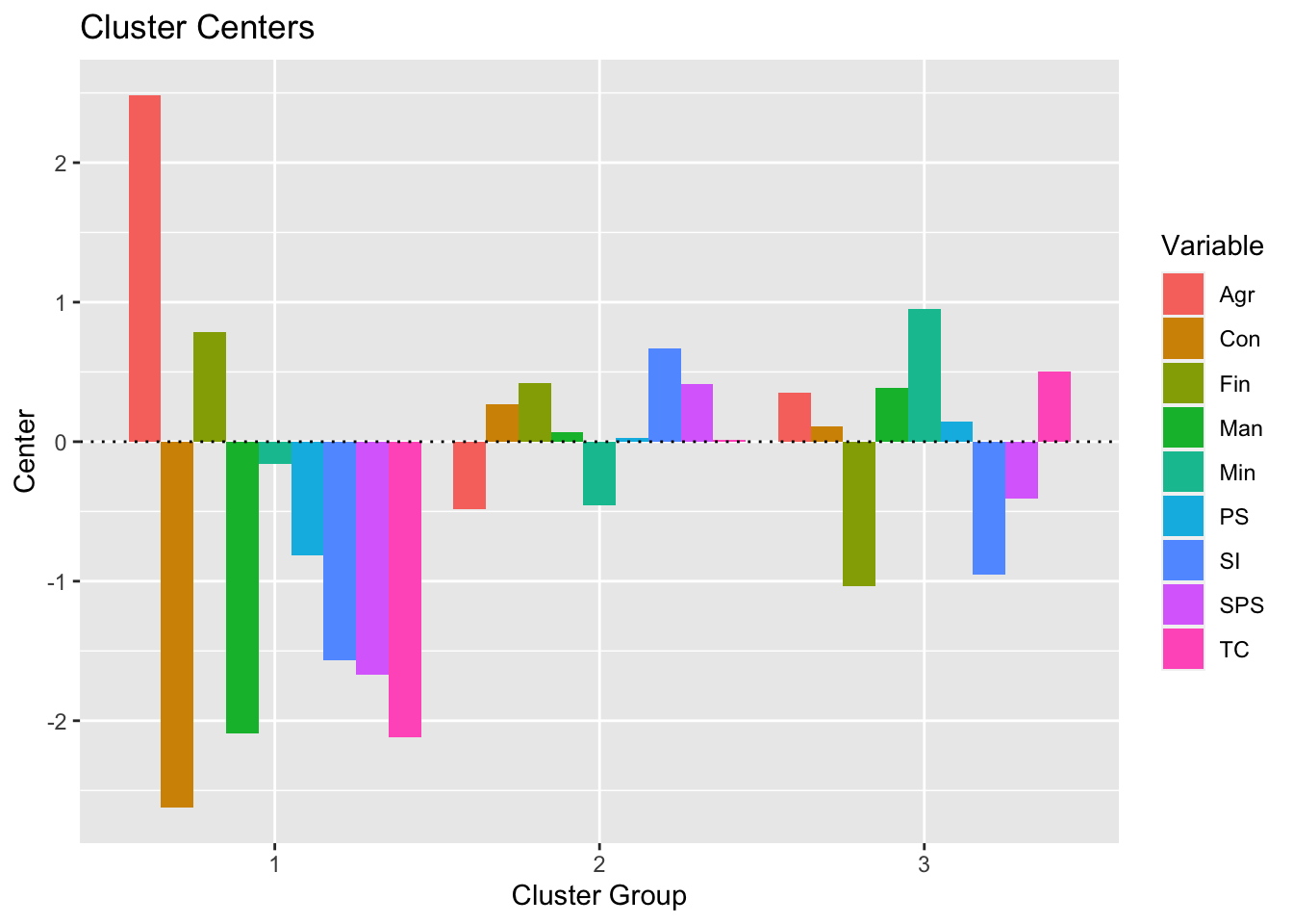
Optimal number of clusters
In order to find the optimal number of clusters for a k-means, it is recommended to choose it based on:
- the context of the problem at hand, for instance if you know that there is a specific number of groups in your data (you have strong expectations or hypotheses, this is option is however subjective), or
- the following four approaches:
- Elbow method (which uses the within cluster sums of squares)
- Average silhouette method
- Gap statistic method
- Consensus-based algorithm
We show the R code for these 4 methods below, more theoretical information can be found here.
Elbow method
The Elbow method looks at the total within-cluster sum of square (WSS) as a function of the number of clusters.
# load required packages
library(factoextra)
library(NbClust)

# Elbow method
fviz_nbclust(Eurojobs, kmeans, method = "wss") +
  geom_vline(xintercept = 4, linetype = 2) + # add line for better visualisation
  labs(subtitle = "Elbow method") # add subtitle
The location of a knee in the plot is usually considered as an indicator of the appropriate number of clusters because it means that adding another cluster does not improve much better the partition. This method seems to suggest 4 clusters.
The Elbow method is sometimes ambiguous and an alternative is the average silhouette method.
Silhouette method
The Silhouette method measures the quality of a clustering and determines how well each point lies within its cluster.
# Silhouette method
fviz_nbclust(Eurojobs, kmeans, method = "silhouette") +
  labs(subtitle = "Silhouette method")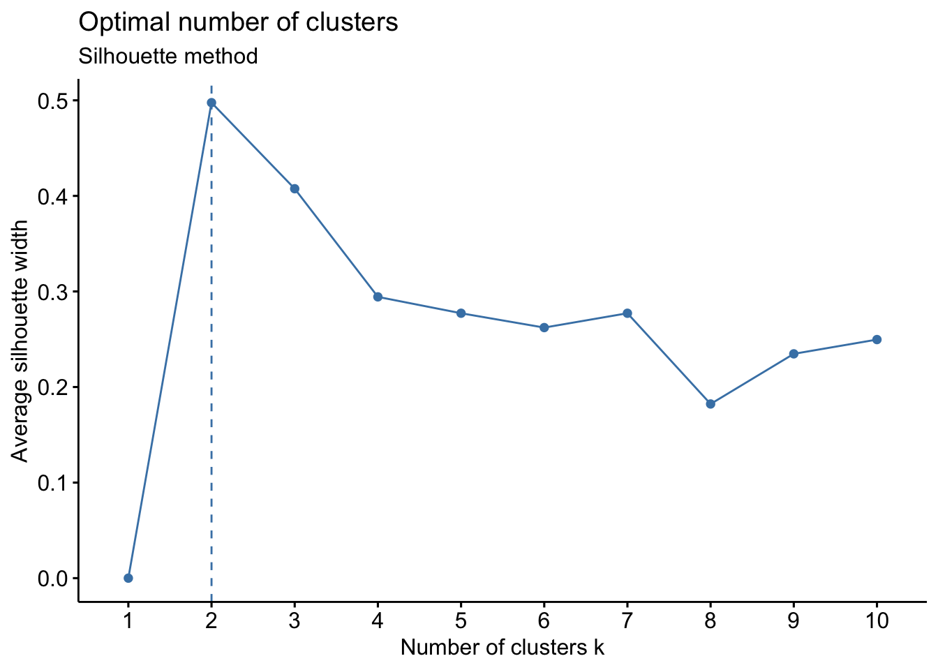
The Silhouette method suggests 2 clusters.
Gap statistic method
# Gap statistic
set.seed(42)
fviz_nbclust(Eurojobs, kmeans,
  nstart = 25,
  method = "gap_stat",
  nboot = 500 # reduce it for lower computation time (but less precise results)
) +
  labs(subtitle = "Gap statistic method")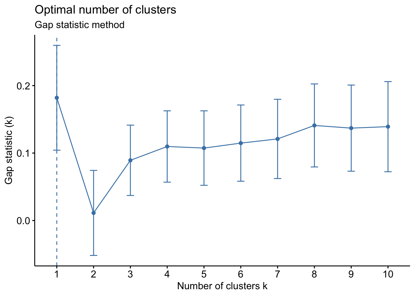
The optimal number of clusters is the one that maximizes the gap statistic. This method suggests only 1 cluster (which is therefore a useless clustering).
As you can see these three methods do not necessarily lead to the same result. Here, the 3 approaches suggest a different number of clusters.
Consensus-based algorithm
Because no method is clearly better, a fourth alternative is to run many methods and take the number of clusters that is the most agreed upon (i.e., find the consensus).
This can easily be done with the n_clusters() function from the {parameters} package:
library(parameters)

n_clust <- n_clusters(Eurojobs,
  package = c("easystats", "NbClust", "mclust"),
  standardize = FALSE
)
n_clust
## # Method Agreement Procedure:
##
## The choice of 3 clusters is supported by 15 (51.72%) methods out of 29 (kl, Ch, Hartigan, CCC, Scott, Marriot, trcovw, Tracew, Rubin, Beale, Ratkowsky, Ball, PtBiserial, Dunn, SDindex).The optimal number of clusters to retain can also be visualized:
plot(n_clust)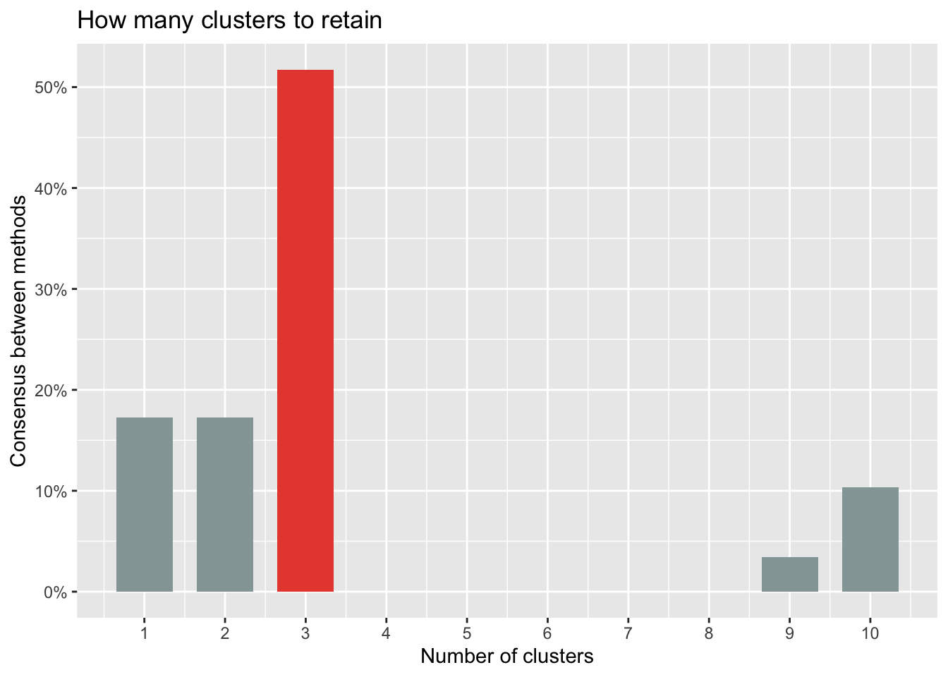
Based on all indices, most methods suggest to retain 3 clusters.
Visualizations
To confirm that your number of classes is indeed optimal, there is a way to evaluate the quality of your clustering via the silhouette plot (which shows the silhouette coefficient on the y axis).
We draw the silhouette plot for 2 clusters, as suggested by the average silhouette method:
library(cluster)

set.seed(42)
km_res <- kmeans(Eurojobs, centers = 2, nstart = 20)

sil <- silhouette(km_res$cluster, dist(Eurojobs))
fviz_silhouette(sil)
## cluster size ave.sil.width
## 1 1 5 0.33
## 2 2 21 0.54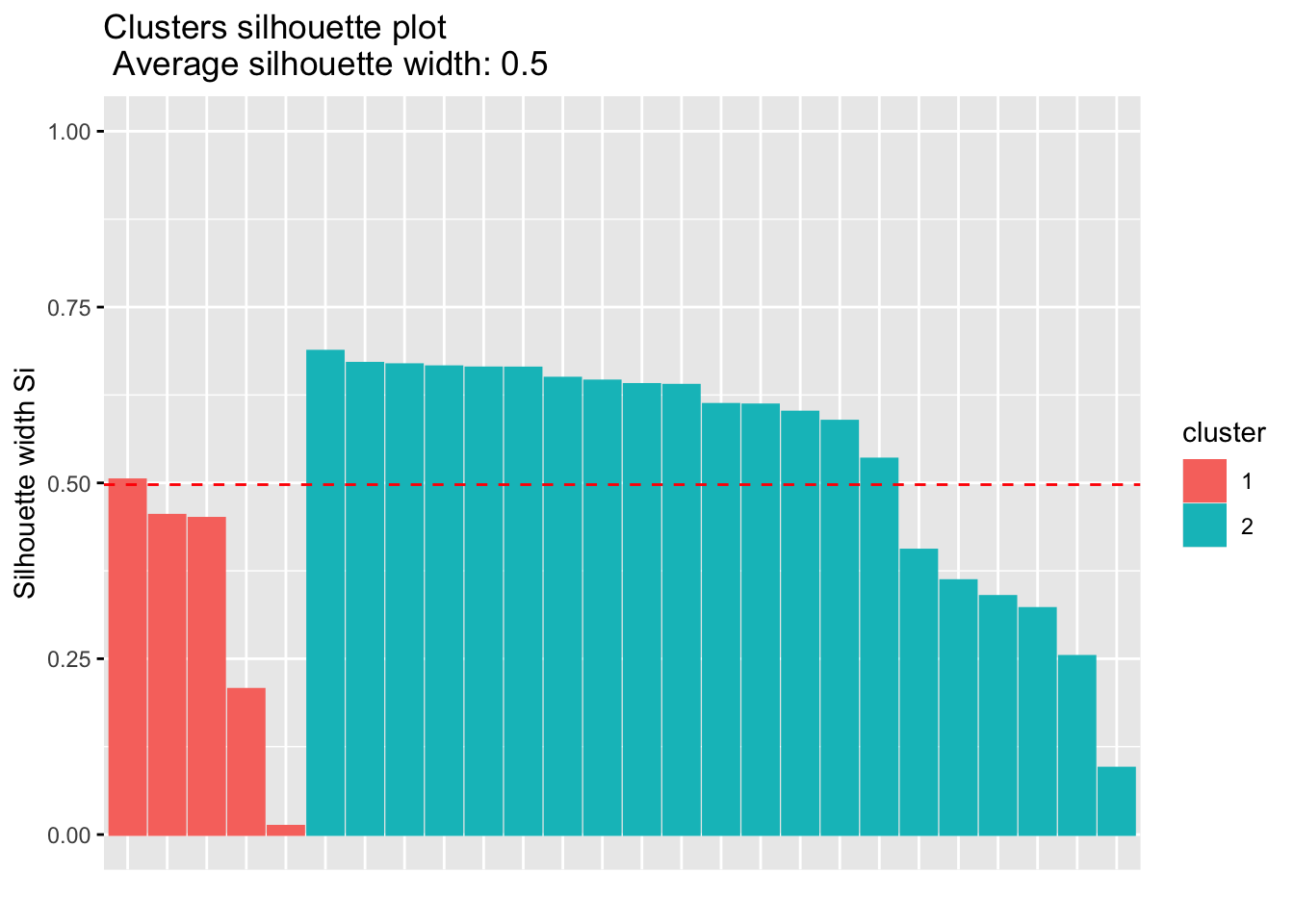
As a reminder, the interpretation of the silhouette coefficient is as follows:
- \(> 0\) means that the observation is well grouped. The closer the coefficient is to 1, the better the observation is grouped.
- \(< 0\) means that the observation has been placed in the wrong cluster.
- \(= 0\) means that the observation is between two clusters.
The silhouette plot above and the average silhouette coefficient help to determine whether your clustering is good or not. If a large majority of the silhouette coefficients are positive, it indicates that the observations are placed in the correct group. This silhouette plot can therefore be used in the choice of the optimal number of classes.
It is also possible to plot clusters by using the fviz_cluster() function. Note that a principal component analysis is performed to represent the variables in a 2 dimensions plane.
library(factoextra)

fviz_cluster(km_res, Eurojobs, ellipse.type = "norm")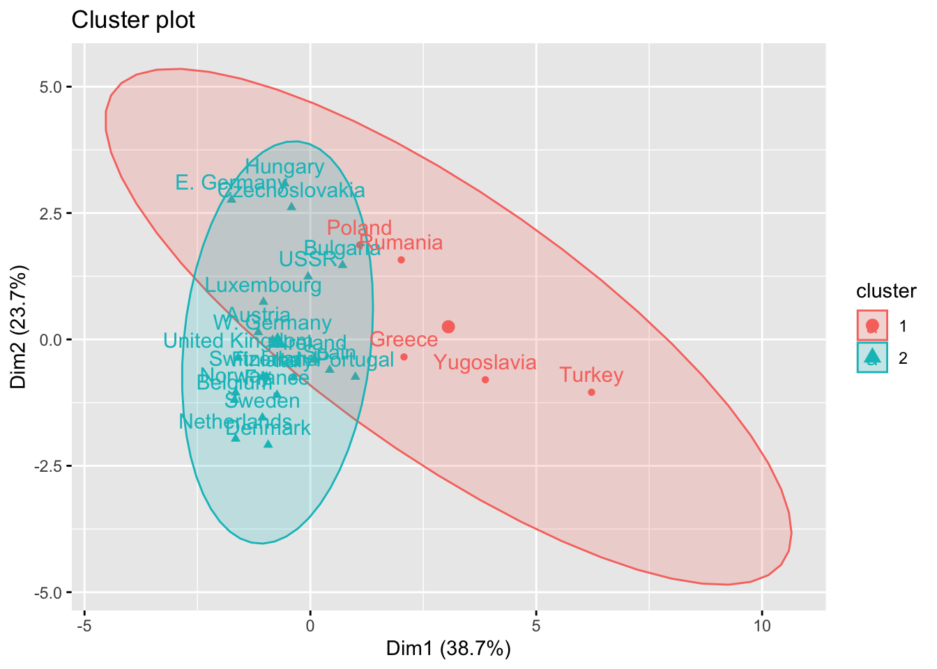
Now that the k-means clustering has been detailed in R, see how to do the algorithm by hand in the following sections.
Manual application and verification in R
Perform by hand the k-means algorithm for the points shown in the graph below, with k = 2 and with the points i = 5 and i = 6 as initial centers. Compute the quality of the partition you just found and then check your answers in R.
Assume that the variables have the same units so there is no need to scale the data.

Solution by hand
Step 1. Here are the coordinates of the 6 points:
| point | x | y |
|---|---|---|
| 1 | 7 | 3 |
| 2 | 4 | 5 |
| 3 | 2 | 4 |
| 4 | 0 | 1 |
| 5 | 9 | 7 |
| 6 | 6 | 8 |
And the initial centers:
- Group 1: point 5 with center (9, 7)
- Group 2: point 6 with center (6, 8)
Step 2. Compute the distance matrix point by point with the Pythagorean theorem. Remind that the distance between point a and point b is found with:
\[\sqrt{(x_a - x_b)^2 + (y_a - y_b)^2}\]
We apply this theorem to each pair of points, to finally have the following distance matrix (rounded to two decimals):
round(dist(X), 2)## 1 2 3 4 5
## 2 3.61
## 3 5.10 2.24
## 4 7.28 5.66 3.61
## 5 4.47 5.39 7.62 10.82
## 6 5.10 3.61 5.66 9.22 3.16Step 3. Based on the distance matrix computed in step 2, we can put each point to its closest group and compute the coordinates of the center.
We first put each point in its closest group:
- point 1 is closer to point 5 than to point 6 because the distance between points 1 and 5 is 4.47 while the distance between points 1 and 6 is 5.10
- point 2 is closer to point 6 than to point 5 because the distance between points 2 and 5 is 5.39 while the distance between points 2 and 6 is 3.61
- point 3 is closer to point 6 than to point 5 because the distance between points 3 and 5 is 7.62 while the distance between points 3 and 6 is 5.66
- point 4 is closer to point 6 than to point 5 because the distance between points 4 and 5 is 10.82 while the distance between points 4 and 6 is 9.22
Note that computing the distances between each point and the points 5 and 6 is sufficient. There is no need to compute the distance between the points 1 and 2 for example, as we compare each point to the initial centers (which are points 5 and 6).
We then compute the coordinates of the centers of the two groups by taking the mean of the coordinates x and y:
- Group 1 includes the points 5 and 1 with (8, 5) as center (\(8 = \frac{9+7}{2}\) and \(5 = \frac{7+3}{2}\))
- Group 2 includes the points 6, 2, 3 and 4 with (3, 4.5) as center (\(3 = \frac{6+4+2+0}{4}\) and \(4.5 = \frac{8+5+4+1}{4}\))
We thus have:
| points | center | |
|---|---|---|
| cluster 1 | 5 & 1 | (8, 5) |
| cluster 2 | 6, 2, 3 & 4 | (3, 4.5) |
Step 4. We make sure that the allocation is optimal by checking that each point is in the nearest cluster. The distance between a point and the center of a cluster is again computed thanks to the Pythagorean theorem. Thus, we have:
| points | Distance to cluster 1 | Distance to cluster 2 |
|---|---|---|
| 1 | 2.24 | 4.27 |
| 2 | 4 | 1.12 |
| 3 | 6.08 | 1.12 |
| 4 | 8.94 | 4.61 |
| 5 | 2.24 | 6.5 |
| 6 | 3.61 | 4.61 |
The minimum distance between the points and the two clusters is colored in green.
We check that each point is in the correct group (i.e., the closest cluster). According to the distance in the table above, point 6 seems to be closer to the cluster 1 than to the cluster 2. Therefore, the allocation is not optimal and point 6 should be reallocated to cluster 1.
Step 5. We compute again the centers of the clusters after this reallocation. The centers are found by taking the mean of the coordinates x and y of the points belonging to the cluster. We thus have:
| points | center | |
|---|---|---|
| cluster 1 | 1, 5 & 6 | (7.33, 6) |
| cluster 2 | 2, 3 & 4 | (2, 3.33) |
where, for instance, 3.33 is simply \(\frac{5+4+1}{3}\).
Step 6. Repeat step 4 until the allocation is optimal. If the allocation is optimal, the algorithm stops. In our example we have:
| points | Distance to cluster 1 | Distance to cluster 2 |
|---|---|---|
| 1 | 3.02 | 5.01 |
| 2 | 3.48 | 2.61 |
| 3 | 5.69 | 0.67 |
| 4 | 8.87 | 3.07 |
| 5 | 1.95 | 7.9 |
| 6 | 2.4 | 5.08 |
All points are correctly allocated to its nearest cluster, so the allocation is optimal and the algorithm stops.
Step 7. State the final partition and the centers. In our example:
| points | center | |
|---|---|---|
| cluster 1 | 1, 5 & 6 | (7.33, 6) |
| cluster 2 | 2, 3 & 4 | (2, 3.33) |
Now that we have the clusters and the final centers, we compute the quality of the partition we just found. Remember that we need to compute the BSS and TSS to find the quality. Below the steps to compute the quality of this partition by k-means, based on this summary table:
| cluster 1 | cluster 2 | ||||
|---|---|---|---|---|---|
| point | x | y | point | x | y |
| 1 | 7 | 3 | 2 | 4 | 5 |
| 5 | 9 | 7 | 3 | 2 | 4 |
| 6 | 6 | 8 | 4 | 0 | 1 |
| mean | 7.33 | 6 | 2 | 3.33 | |
Step 1. Compute the overall mean of the x and y coordinates:
\[\overline{\overline{x}} = \frac{7+4+2+0+9+6}{12} \\ \frac{+3+5+4+1+7+8}{12} \\ = 4.67\]
Step 2. Compute TSS and WSS:
\[TSS = (7-4.67)^2 + (4-4.67)^2 + (2-4.67)^2 \\ + (0-4.67)^2 + (9-4.67)^2 + (6-4.67)^2 \\ + (3-4.67)^2 + (5-4.67)^2 + (4-4.67)^2 \\ + (1-4.67)^2 + (7-4.67)^2 + (8-4.67)^2 \\ = 88.67\]
Regarding WSS, it is splitted between cluster 1 and cluster 2. For cluster 1:
\[WSS[1] = (7-7.33)^2 + (9 - 7.33)^2 \\ + (6 - 7.33)^2 + (3-6)^2 \\ + (7-6)^2 + (8-6)^2 \\ = 18.67\]
For cluster 2:
\[WSS[2] = (4-2)^2 + (2-2)^2 + (0-2)^2 \\ + (5-3.33)^2 + (4-3.33)^2 + (1-3.33)^2 \\ = 16.67\]
And the total WSS is
\[\begin{align} WSS &= WSS[1] + WSS[2] \\ &= 18.67 + 16.67 \\ &= 35.34 \end{align}\]
To find the BSS:
\[\begin{align} BSS &= TSS - WSS \\ &= 88.67 - 35.34 \\ &= 53.33 \end{align}\]
Finally, the quality of the partition is:
\[Quality = \frac{BSS}{TSS} = \frac{53.33}{88.67} = 0.6014\]
So the quality of the partition is 60.14%.
We are now going to verify all these solutions (the partition, the final centers and the quality) in R.
Solution in R
As you can imagine, the solution in R us much shorter and requires much less computation on the user side. We first need to enter the data as a matrix or dataframe:
X <- matrix(c(7, 3, 4, 5, 2, 4, 0, 1, 9, 7, 6, 8),
  nrow = 6, byrow = TRUE
)
X # display the coordinates of the points
## [,1] [,2]
## [1,] 7 3
## [2,] 4 5
## [3,] 2 4
## [4,] 0 1
## [5,] 9 7
## [6,] 6 8We now perform the k-means via the kmeans() function with the point 5 and 6 as initial centers:
# take rows 5 and 6 of the X matrix as initial centers
res.k <- kmeans(X,
  centers = X[c(5, 6), ],
  algorithm = "Lloyd"
)
Unlike in the previous application with the dataset Eurojobs.csv where the initial centers are randomly chosen by R, in this second application we want to specify which points are going to be the two initial centers. For this, we need to set centers = X[c(5,6), ] to indicate that that there are 2 centers, and that they are going to be the points 5 and 6 (see a reminder on how to subset a dataframe if needed).
The reason for adding the argument algorithm = "Lloyd" can be found in the usage of the R function kmeans(). In fact, there are several variants of the k-means algorithm. The default choice is the Hartigan and Wong (1979) version, which is more sophisticated than the basic version detailed in the solution by hand. By using the original version of Lloyd (1982), we find the same solution in R and by hand. For more information, you can consult the documentation of the kmeans() function (via ?kmeans or help(kmeans)) and read the articles mentioned.
The solution in R is then found by extracting
- the partition with
$cluster:
res.k$cluster## [1] 1 2 2 2 1 1Points 1, 5 and 6 belong to cluster 1, points 2, 3 and 4 belong to cluster 2.
- the coordinates of the final centers with
$centers:
# We extract the coordinates of the 2 final centers, rounded to 2 decimals
round(res.k$centers, digits = 2)
## [,1] [,2]
## 1 7.33 6.00
## 2 2.00 3.33- and then the quality of the partition by dividing the BSS to the TSS:
res.k$betweenss / res.k$totss## [1] 0.6015038The 3 results are equal to what we found by hand (except the quality which is slightly different due to rounding).
Hierarchical clustering
Remind that the difference with the partition by k-means is that for hierarchical clustering, the number of classes is not specified in advance. Hierarchical clustering will help to determine the optimal number of clusters.
Before applying hierarchical clustering by hand and in R, let’s see how the ascending hierarchical clustering works step by step:
- It starts by putting every point in its own cluster, so each cluster is a singleton
- It then merges the 2 points that are closest to each other based on the distances from the distance matrix. The consequence is that there is one less cluster
- It then recalculates the distances between the new and old clusters and save them in a new distance matrix which will be used in the next step
- Finally, steps 1 and 2 are repeated until all clusters are merged into one single cluster including all points.
There are 5 main methods to measure the distance between clusters, referred as linkage methods:
- Single linkage: computes the minimum distance between clusters before merging them.
- Complete linkage: computes the maximum distance between clusters before merging them.
- Average linkage: computes the average distance between clusters before merging them.
- Centroid linkage: calculates centroids for both clusters, then computes the distance between the two before merging them.
- Ward’s (minimum variance) criterion: minimizes the total within-cluster variance and find the pair of clusters that leads to minimum increase in total within-cluster variance after merging.
In the following sections, only the three first linkage methods are presented (first by hand and then the results are verified in R).
Application 3: hierarchical clustering
Data
Using the data from the graph and the table below, we perform by hand the 3 algorithms (single, complete and average linkage) and we draw the dendrograms. Then we check our answers in R.
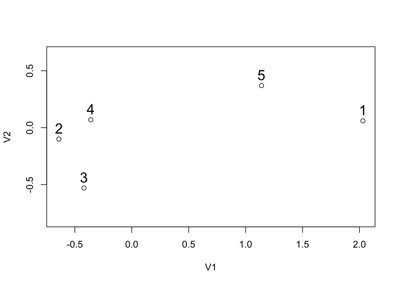
##      V1    V2
## 1  2.03  0.06
## 2 -0.64 -0.10
## 3 -0.42 -0.53
## 4 -0.36  0.07
## 5  1.14  0.37
We assume that the variables have the same units so there is no need to scale the data.
Solution by hand
Step 1. For all 3 algorithms, we first need to compute the distance matrix between the 5 points thanks to the Pythagorean theorem. Remind that the distance between point a and point b is found with:
\[\sqrt{(x_a - x_b)^2 + (y_a - y_b)^2}\]
We apply this theorem to each pair of points, to finally have the following distance matrix (rounded to three decimals):
##       1     2     3     4
## 2 2.675
## 3 2.520 0.483
## 4 2.390 0.328 0.603
## 5 0.942 1.841 1.801 1.530
Single linkage
Step 2. From the distance matrix computed in step 1, we see that the smallest distance = 0.328 between points 2 and 4. 0.328 corresponds to the first height (more on this later when drawing the dendrogram). Since points 2 and 4 are the closest to each other, these 2 points are put together to form a single group. The groups are thus: 1, 2 & 4, 3 and 5. The new distances between the group 2 & 4 and all other points are now:
| 1 | 2 & 4 | 3 | 5 | |
|---|---|---|---|---|
| 1 | 0 | |||
| 2 & 4 | 2.390 | 0 | ||
| 3 | 2.520 | 0.483 | 0 | |
| 5 | 0.942 | 1.530 | 1.801 | 0 |
To construct this new distance matrix, proceed point by point:
- the distance between points 1 and 3 has not changed, so the distance is unchanged compared to the initial distance matrix (found in step 1), which was 2.520
- same goes for the distance between points 1 and 5 and points 3 and 5; the distances are the same than in the initial distance matrix since the points have not changed
- the distance between points 1 and 2 & 4 has changed since points 2 & 4 are now together
- since we are applying the single linkage criterion, the new distance between points 1 and 2 & 4 corresponds to the minimum distance between the distance between points 1 and 2 and the distance between points 1 and 4
- the initial distance between points 1 and 2 is 2.675 and the initial distance between points 1 and 4 is 2.390
- therefore, the minimum distance between these two distances is 2.390
- 2.390 is thus the new distance between points 1 and 2 & 4
- we apply the same process for points 3 and 2 & 4: the initial distance between points 3 and 2 is 0.483 and the initial distance between points 3 and 4 is 0.603. The minimum distance between these 2 distances is 0.483 so the new distance between points 3 and 2 & 4 is 0.483
- follow the same process for all other points
Step 3. Based on the distance matrix in step 2, the smallest distance is 0.483 between points 3 and 2 & 4 (the second height for the dendrogram). Since points 3 and 2 & 4 are the closest to each other, they are combined to form a new group, the group 2 & 3 & 4. The groups are thus: 1, 2 & 3 & 4 and 5. We construct the new distance matrix based on the same process detailed in step 2:
| 1 | 2 & 3 & 4 | 5 | |
|---|---|---|---|
| 1 | 0 | ||
| 2 & 3 & 4 | 2.390 | 0 | |
| 5 | 0.942 | 1.530 | 0 |
- points 1 and 5 have not change, so the distance between these two points are the same than in previous step
- from step 2 we see that the distance between points 1 and 2 & 4 is 2.390 and the distance between points 1 and 3 is 2.520
- since we apply the single linkage criterion, we take the minimum distance, which is 2.390
- the distance between points 1 and 2 & 3 & 4 is thus 2.390
- same process for points 5 and 2 & 3 & 4
Step 4. Based on the distance matrix in step 3, the smallest distance is 0.942 between points 1 and 5 (the third height in the dendrogram). Since points 1 and 5 are the closest to each other, they are combined to form a new group, the group 1 & 5. The groups are thus: 1 & 5 and 2 & 3 & 4. We construct the new distance matrix based on the same process detailed in steps 2 and 3:
| 1 & 5 | 2 & 3 & 4 | |
|---|---|---|
| 1 & 5 | 0 | |
| 2 & 3 & 4 | 1.530 | 0 |
- the only distance left to compute is the distance between points 1 & 5 and 2 & 3 & 4
- from the previous step we see that the distance between points 1 and 2 & 3 & 4 is 2.390 and the distance between points 5 and 2 & 3 & 4 is 1.530
- since we apply the single linkage criterion, we take the minimum distance, which is 1.530
- the distance between points 1 & 5 and 2 & 3 & 4 is thus 1.530
Step 5. The final combination of points is the combination of points 1 & 5 and 2 & 3 & 4, with a final height of 1.530. Heights are used to draw the dendrogram in the sixth and final step.
Step 6. Draw the dendrogram thanks to the combination of points and heights found above. Remember that:
- the first combination of points was between points 2 and 4, with a height of 0.328
- the second combination was between points 3 and 2 & 4 with a height of 0.483
- the third combination was between points 1 and 5 with a height of 0.942
- the final combination was between points 1 & 5 and 2 & 3 & 4 with a height of 1.530
- this is exactly what is illustrated in the following dendrogram:
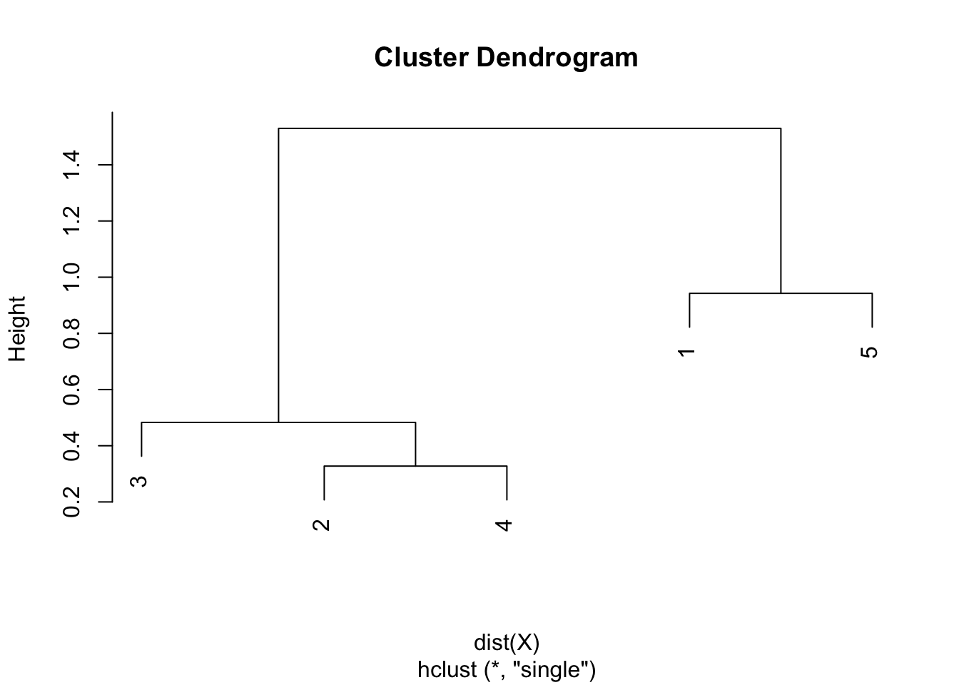
In hierarchical clustering, dendrograms are used to show the sequence of combinations of the clusters. The distances of merge between clusters, called heights, are illustrated on the y-axis.
Complete linkage
Complete linkage is quite similar to single linkage, except that instead of taking the smallest distance when computing the new distance between points that have been grouped, the maximum distance is taken.
The steps to perform the hierarchical clustering with the complete linkage (maximum) are detailed below.
Step 1. Step 1 is exactly the same than for single linkage, that is, we compute the distance matrix of the 5 points thanks to the Pythagorean theorem. This gives us the following distance matrix:
##       1     2     3     4
## 2 2.675
## 3 2.520 0.483
## 4 2.390 0.328 0.603
## 5 0.942 1.841 1.801 1.530
Step 2. From the distance matrix computed in step 1, we see that the smallest distance = 0.328 between points 2 and 4. It is important to note that even if we apply the complete linkage, in the distance matrix the points are brought together based on the smallest distance. This is the case for all 3 algorithms. The difference between the 3 algorithms lies in how to compute the new distances between the new combination of points (the single linkage takes the minimum between the distances, the complete linkage takes the maximum distance and the average linkage takes the average distance). 0.328 corresponds to the first height (which will be used when drawing the dendrogram). Since points 2 and 4 are the closest to each other, these 2 points are put together to form a single group. The groups are thus: 1, 2 & 4, 3 and 5. The new distances between the group 2 & 4 and all other points are now:
| 1 | 2 & 4 | 3 | 5 | |
|---|---|---|---|---|
| 1 | 0 | |||
| 2 & 4 | 2.675 | 0 | ||
| 3 | 2.520 | 0.603 | 0 | |
| 5 | 0.942 | 1.841 | 1.801 | 0 |
To construct this new distance matrix, proceed point by point as we did for single linkage:
- the distance between points 1 and 3 has not changed, so the distance is unchanged compared to the initial distance matrix (found in step 1), which was 2.520
- same goes for the distance between points 1 and 5 and points 3 and 5; the distances are the same than in the initial distance matrix since the points have not changed
- the distance between points 1 and 2 & 4 has changed since points 2 & 4 are now together
- since we are applying the complete linkage criterion, the new distance between points 1 and 2 & 4 corresponds to the maximum distance between the distance between points 1 and 2 and the distance between points 1 and 4
- the initial distance between points 1 and 2 is 2.675 and the initial distance between points 1 and 4 is 2.390
- therefore, the maximum distance between these two distances is 2.675
- 2.675 is thus the new distance between points 1 and 2 & 4
- we apply the same process for points 3 and 2 & 4: the initial distance between points 3 and 2 is 0.483 and the initial distance between points 3 and 4 is 0.603. The maximum distance between these 2 distances is 0.603 so the new distance between points 3 and 2 & 4 is 0.603
- follow the same process for all other points
Step 3. Based on the distance matrix in step 2, the smallest distance is 0.603 between points 3 and 2 & 4 (the second height for the dendrogram). Since points 3 and 2 & 4 are the closest to each other, they are combined to form a new group, the group 2 & 3 & 4. The groups are thus: 1, 2 & 3 & 4 and 5. We construct the new distance matrix based on the same process detailed in step 2:
| 1 | 2 & 3 & 4 | 5 | |
|---|---|---|---|
| 1 | 0 | ||
| 2 & 3 & 4 | 2.675 | 0 | |
| 5 | 0.942 | 1.841 | 0 |
- points 1 and 5 have not change, so the distance between these two points are the same than in previous step
- from step 2 we see that the distance between points 1 and 2 & 4 is 2.675 and the distance between points 1 and 3 is 2.520
- since we apply the complete linkage criterion, we take the maximum distance, which is 2.675
- the distance between points 1 and 2 & 3 & 4 is thus 2.675
- same process for points 5 and 2 & 3 & 4
Step 4. Based on the distance matrix in step 3, the smallest distance is 0.942 between points 1 and 5 (the third height in the dendrogram). Since points 1 and 5 are the closest to each other, they are combined to form a new group, the group 1 & 5. The groups are thus: 1 & 5 and 2 & 3 & 4. We construct the new distance matrix based on the same process detailed in steps 2 and 3:
| 1 & 5 | 2 & 3 & 4 | |
|---|---|---|
| 1 & 5 | 0 | |
| 2 & 3 & 4 | 2.675 | 0 |
- the only distance left to compute is the distance between points 1 & 5 and 2 & 3 & 4
- from the previous step we see that the distance between points 1 and 2 & 3 & 4 is 2.675 and the distance between points 5 and 2 & 3 & 4 is 1.841
- since we apply the complete linkage criterion, we take the maximum distance, which is 2.675
- the distance between points 1 & 5 and 2 & 3 & 4 is thus 2.675
Step 5. The final combination of points is the combination of points 1 & 5 and 2 & 3 & 4, with a final height of 2.675. Heights are used to draw the dendrogram in the sixth and final step.
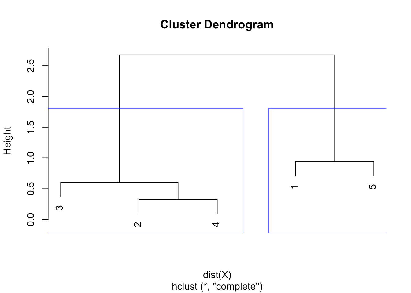
Step 6. Draw the dendrogram thanks to the combination of points and heights found above. Remember that:
- the first combination of points was between points 2 and 4, with a height of 0.328
- the second combination was between points 3 and 2 & 4 with a height of 0.603
- the third combination was between points 1 and 5 with a height of 0.942
- the final combination was between points 1 & 5 and 2 & 3 & 4 with a height of 2.675
- this is exactly what is illustrated in the following dendrogram:

Average linkage
With the average linkage criterion, it is not the minimum nor the maximum distance that is taken when computing the new distance between points that have been grouped, but it is, as you guessed by now, the average distance between the points.
The steps to perform the hierarchical clustering with the average linkage are detailed below.
Step 1. Step 1 is exactly the same than for single and complete linkage, that is, we compute the distance matrix of the 5 points thanks to the Pythagorean theorem. This gives us the following distance matrix:
##       1     2     3     4
## 2 2.675
## 3 2.520 0.483
## 4 2.390 0.328 0.603
## 5 0.942 1.841 1.801 1.530
Step 2. From the distance matrix computed in step 1, we see that the smallest distance = 0.328 between points 2 and 4. It is important to note that even if we apply the average linkage, in the distance matrix the points are brought together based on the smallest distance. This is the case for all 3 algorithms. The difference between the 3 algorithms lies in how to compute the new distances between the new combination of points (the single linkage takes the minimum between the distances, the complete linkage takes the maximum distance and the average linkage takes the average distance). 0.328 corresponds to the first height (which will be used when drawing the dendrogram). Since points 2 and 4 are the closest to each other, these 2 points are put together to form a single group. The groups are thus: 1, 2 & 4, 3 and 5. The new distances between the group 2 & 4 and all other points are now:
| 1 | 2 & 4 | 3 | 5 | |
|---|---|---|---|---|
| 1 | 0 | |||
| 2 & 4 | 2.5325 | 0 | ||
| 3 | 2.520 | 0.543 | 0 | |
| 5 | 0.942 | 1.6855 | 1.801 | 0 |
To construct this new distance matrix, proceed point by point as we did for the two previous criteria:
- the distance between points 1 and 3 has not changed, so the distance is unchanged compared to the initial distance matrix (found in step 1), which was 2.520
- same goes for the distance between points 1 and 5 and points 3 and 5; the distances are the same than in the initial distance matrix since the points have not changed
- the distance between points 1 and 2 & 4 has changed since points 2 & 4 are now together
- since we are applying the average linkage criterion, the new distance between points 1 and 2 & 4 corresponds to the average distance between the distance between points 1 and 2 and the distance between points 1 and 4
- the initial distance between points 1 and 2 is 2.675 and the initial distance between points 1 and 4 is 2.390
- therefore, the average distance between these two distances is \(\frac{2.675 + 2.390}{2} = 2.5325\)
- 2.5325 is thus the new distance between points 1 and 2 & 4
- we apply the same process for points 3 and 2 & 4: the initial distance between points 3 and 2 is 0.483 and the initial distance between points 3 and 4 is 0.603. The average distance between these 2 distances is 0.543 so the new distance between points 3 and 2 & 4 is 0.543
- follow the same process for all other points
Step 3. Based on the distance matrix in step 2, the smallest distance is 0.543 between points 3 and 2 & 4 (the second height for the dendrogram). Since points 3 and 2 & 4 are the closest to each other, they are combined to form a new group, the group 2 & 3 & 4. The groups are thus: 1, 2 & 3 & 4 and 5. We construct the new distance matrix based on the same process detailed in step 2:
| 1 | 2 & 3 & 4 | 5 | |
|---|---|---|---|
| 1 | 0 | ||
| 2 & 3 & 4 | 2.528333 | 0 | |
| 5 | 0.942 | 1.724 | 0 |
- points 1 and 5 have not change, so the distance between these two points are the same than in previous step
- from step 2 we see that the distance between points 1 and 2 & 4 is 2.5325 and the distance between points 1 and 3 is 2.520
- since we apply the average linkage criterion, we take the average distance
- however, we have to take into the consideration that there are 2 points in the group 2 & 4, while there is only one point in the group 3
- the average distance for the distance between 1 and 2 & 3 & 4 is thus: \(\frac{(2 \cdot 2.5325) + (1 \cdot 2.520)}{3} = 2.528333\)
- same process for points 5 and 2 & 3 & 4: \(\frac{(2 \cdot 1.6855) + (1 \cdot 1.801)}{3} = 1.724\)
Step 4. Based on the distance matrix in step 3, the smallest distance is 0.942 between points 1 and 5 (the third height in the dendrogram). Since points 1 and 5 are the closest to each other, they are combined to form a new group, the group 1 & 5. The groups are thus: 1 & 5 and 2 & 3 & 4. We construct the new distance matrix based on the same process detailed in steps 2 and 3:
| 1 & 5 | 2 & 3 & 4 | |
|---|---|---|
| 1 & 5 | 0 | |
| 2 & 3 & 4 | 2.126167 | 0 |
- the only distance left to compute is the distance between points 1 & 5 and 2 & 3 & 4
- from the previous step we see that the distance between points 1 and 2 & 3 & 4 is 2.528333 and the distance between points 5 and 2 & 3 & 4 is 1.724
- since we apply the average linkage criterion, we take the average distance, which is \(\frac{2.528333 + 1.724}{2} = 2.126167\)
- the distance between points 1 & 5 and 2 & 3 & 4 is thus 2.126167
Step 5. The final combination of points is the combination of points 1 & 5 and 2 & 3 & 4, with a final height of 2.126167. Heights are used to draw the dendrogram in the sixth and final step.
Step 6. Draw the dendrogram thanks to the combination of points and heights found above. Remember that:
- the first combination of points was between points 2 and 4, with a height of 0.328
- the second combination was between points 3 and 2 & 4 with a height of 0.543
- the third combination was between points 1 and 5 with a height of 0.942
- the final combination was between points 1 & 5 and 2 & 3 & 4 with a height of 2.126167
- this is exactly what is illustrated in the following dendrogram:

Solution in R
To perform the hierarchical clustering with any of the 3 criterion in R, we first need to enter the data (in this case as a matrix format, but it can also be entered as a dataframe):
X <- matrix(c(2.03, 0.06, -0.64, -0.10, -0.42, -0.53, -0.36, 0.07, 1.14, 0.37),
  nrow = 5, byrow = TRUE
)
Single linkage
We can apply the hierarchical clustering with the single linkage criterion thanks to the hclust() function with the argument method = "single":
# Hierarchical clustering: single linkage
hclust <- hclust(dist(X), method = "single")
Note that the hclust() function requires a distance matrix. If your data is not already a distance matrix (like in our case, as the matrix X corresponds to the coordinates of the 5 points), you can transform it into a distance matrix with the dist() function.
We can now extract the heights and plot the dendrogram to check our results by hand found above:
round(hclust$height, 3)## [1] 0.328 0.483 0.942 1.530plot(hclust)
As we can see from the dendrogram, the combination of points and the heights are the same than the ones obtained by hand.
Optimal number of clusters
Remember that hierarchical clustering is used to determine the optimal number of clusters. This optimal number of clusters can be determined thanks to the dendrogram. For this, we usually look at the largest difference of heights:
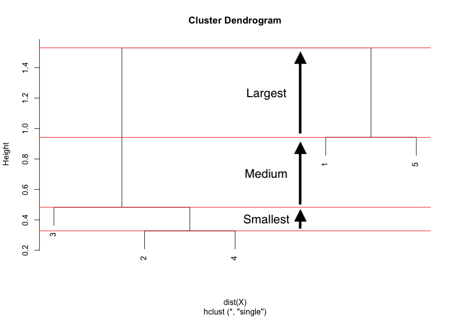
The largest difference of heights in the dendrogram occurs before the final combination, that is, before the combination of the group 2 & 3 & 4 with the group 1 & 5. To determine the optimal number of clusters, simply count how many vertical lines you see within this largest difference. In our case, the optimal number of clusters is thus 2.
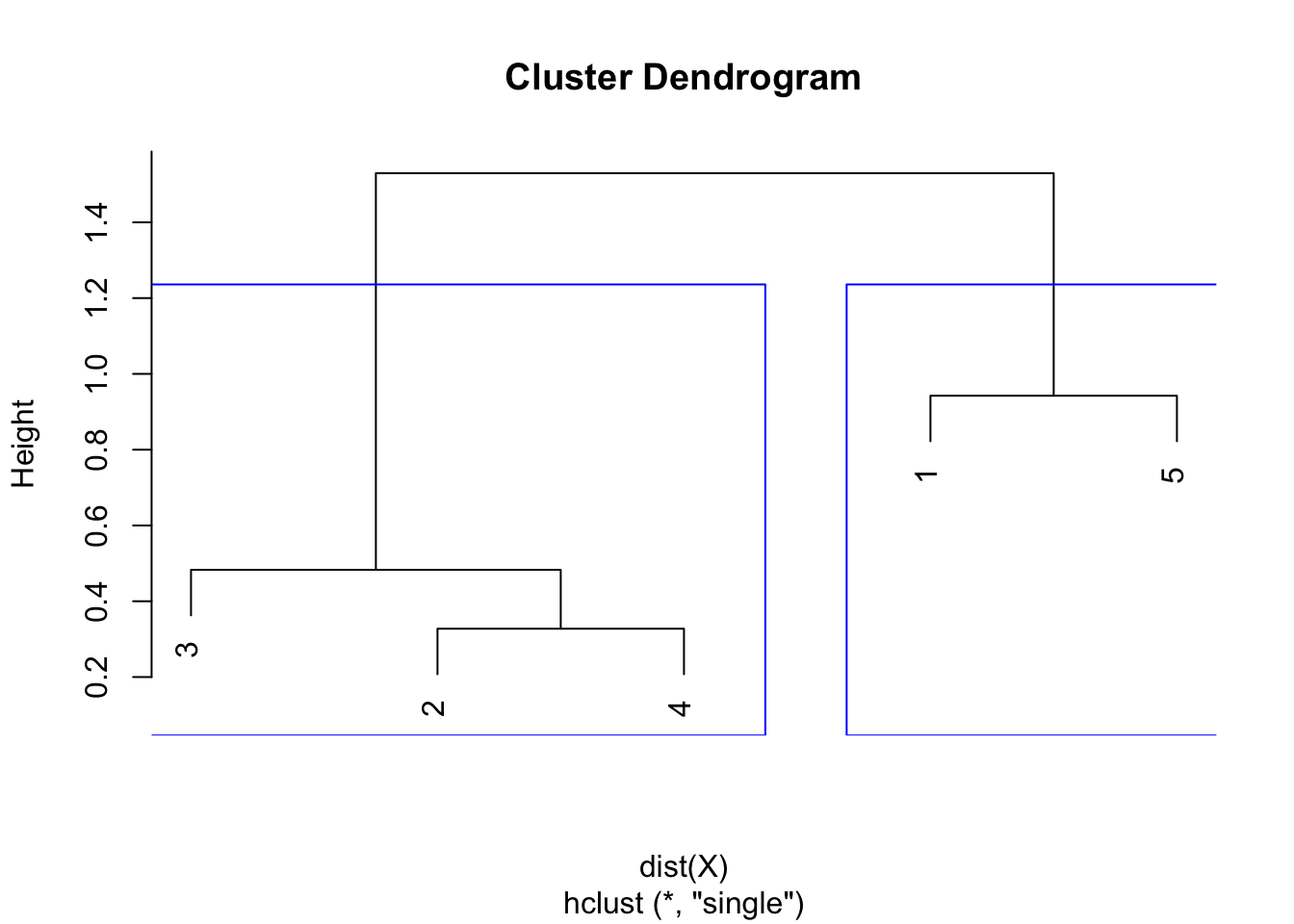
In R, we can even highlight these two clusters directly in the dendrogram with the rect.hclust() function:
plot(hclust)
rect.hclust(hclust,
  k = 2, # k is used to specify the number of clusters
  border = "blue"
)
Note that determining the optimal number of clusters via the dendrogram is not specific to the single linkage, it can be applied to other linkage methods too!
Below another figure explaining how to determine the optimal number of clusters:
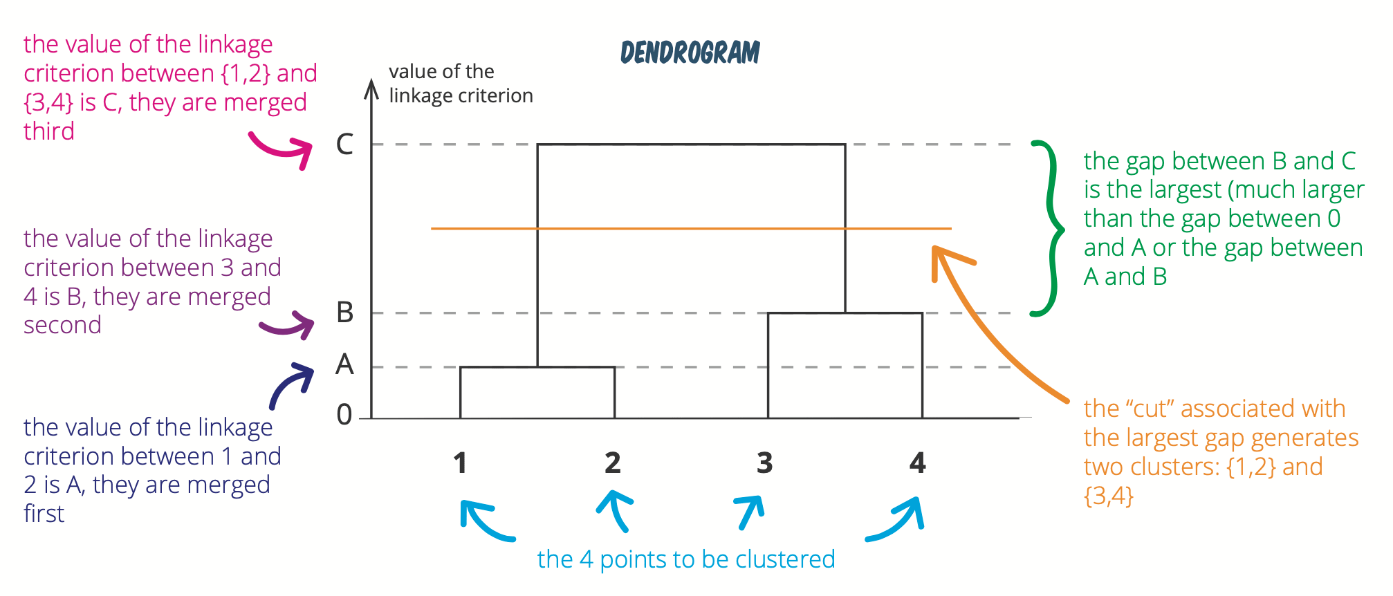
(See this hierarchical clustering cheatsheet for more visualizations like this.)
Finally, we could also determine the optimal number of cluster thanks to a barplot of the heights (stored in $height of the clustering output):
barplot(hclust$height,
  names.arg = (nrow(X) - 1):1 # show the number of cluster below each bars
)
Again, look for the largest jump of heights. In our case, the largest jump is from 1 to 2 classes. Therefore, the optimal number of classes is 2.
Note that determining the number of clusters using the dendrogram or barplot is not a strict rule. You can also consider other methods such as the silhouette plot, elbow plot or some numerical measures like Dunn’s index, Hubert’s gamma, etc., which show the variation of the error with the number of clusters (k), and you choose the value of k where the error is smallest. Furthermore, measuring the goodness of clusters can be done thanks to the Dunn’s Index (the higher the index, the better).
However, these methods are beyond the scope of this article and the method presented with the dendrogram is generally sufficient. See more detailed information in this article.
Note that hierarchical clustering is a bit different than k-means in the sense that is does not return a vector containing the information about which cluster the observations belong to. Instead, it creates a hierarchical structure (a dendrogram), a tree from which we can cut branches to get a given number of clusters. This information can be found via the cutree() function:
clust <- cutree(hclust,
  k = 2
)
clust
## [1] 1 2 2 2 1We see that:
- points 1 and 5 belong to the cluster 1
- points 2, 3 and 4 belong to the cluster 2
This is exactly what was drawn in the dendrogram above, and if needed, this information can be added to the initial data:
X_clust <- cbind(X, clust)
X_clust
## clust
## [1,] 2.03 0.06 1
## [2,] -0.64 -0.10 2
## [3,] -0.42 -0.53 2
## [4,] -0.36 0.07 2
## [5,] 1.14 0.37 1Complete linkage
We can apply the hierarchical clustering with the complete linkage criterion thanks to the hclust() function with the argument method = "complete":
# Hierarchical clustering: complete linkage
hclust <- hclust(dist(X), method = "complete")
Note that the hclust() function requires a distance matrix. If your data is not already a distance matrix (like in our case, as the matrix X corresponds to the coordinates of the 5 points), you can transform it into a distance matrix with the dist() function.
We can now extract the heights and plot the dendrogram to check our results by hand found above:
round(hclust$height, 3)## [1] 0.328 0.603 0.942 2.675plot(hclust)
As we can see from the dendrogram, the combination of points and the heights are the same than the ones obtained by hand.
Similar to the single linkage, the largest difference of heights in the dendrogram occurs before the final combination, that is, before the combination of the group 2 & 3 & 4 with the group 1 & 5. In this case, the optimal number of clusters is thus 2. In R, we can even highlight these two clusters directly in the dendrogram with the rect.hclust() function:
plot(hclust)
rect.hclust(hclust,
  k = 2, # k is used to specify the number of clusters
  border = "blue"
)
Average linkage
We can apply the hierarchical clustering with the average linkage criterion thanks to the hclust() function with the argument method = "average":
# Hierarchical clustering: average linkage
hclust <- hclust(dist(X), method = "average")
Note that the hclust() function requires a distance matrix. If your data is not already a distance matrix (like in our case, as the matrix X corresponds to the coordinates of the 5 points), you can transform it into a distance matrix with the dist() function.
We can now extract the heights and plot the dendrogram to check our results by hand found above:
round(hclust$height, 3)## [1] 0.328 0.543 0.942 2.126plot(hclust)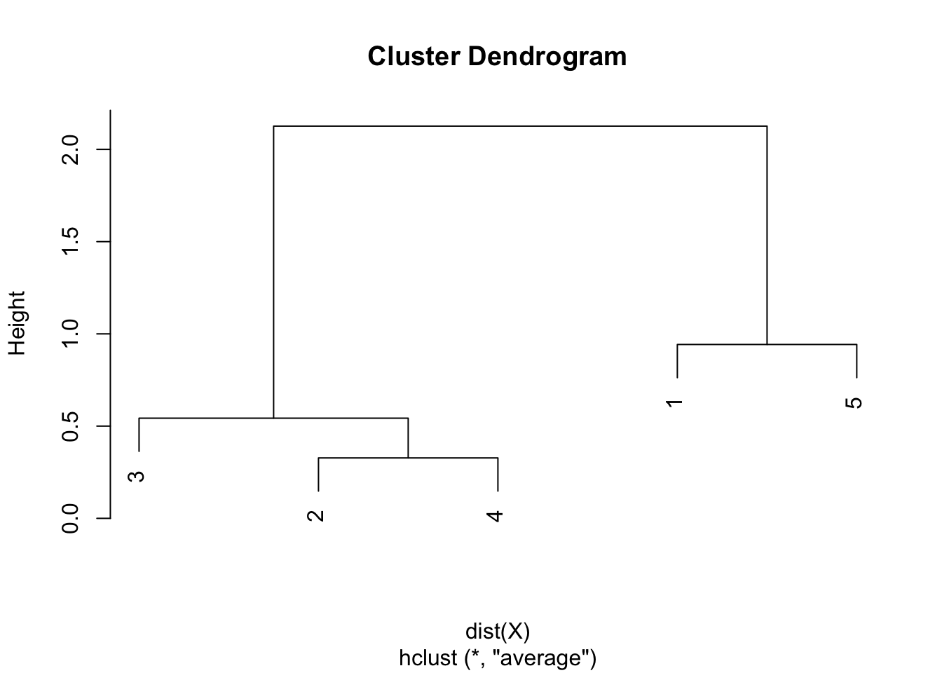
As we can see from the dendrogram, the combination of points and the heights are the same than the ones obtained by hand.
Like the single and complete linkages, the largest difference of heights in the dendrogram occurs before the final combination, that is, before the combination of the group 2 & 3 & 4 with the group 1 & 5. In this case, the optimal number of clusters is thus 2. In R, we can even highlight these two clusters directly in the dendrogram with the rect.hclust() function:
plot(hclust)
rect.hclust(hclust,
  k = 2, # k is used to specify the number of clusters
  border = "blue"
)
k-means versus hierarchical clustering
Clustering is rather a subjective statistical analysis and there can be more than one appropriate algorithm, depending on the dataset at hand or the type of problem to be solved. So choosing between k-means and hierarchical clustering is not always easy. Moreover, no method is better than the other, each come with their sets of limitations and benefits.
If you have a good reason to think that there is a specific number of clusters in your dataset (for example if you would like to distinguish diseased and healthy patients depending on some characteristics but you do not know in which group patients belong to), you should probably opt for the k-means clustering as this technique is used when the number of groups is specified in advance. If you do not have any reason to believe there is a certain number of groups in your dataset (for instance in marketing when trying to distinguish clients without any prior belief on the number of different types of customers), then you should probably opt for the hierarchical clustering to determine in how many clusters your data should be divided.
In addition to this, if you are still undecided note that, on the one hand, with a large number of variables, k-means may be computationally faster than hierarchical clustering if the number of clusters is small. On the other hand, the result of a hierarchical clustering is a structure that is more informative and interpretable than the unstructured set of flat clusters returned by k-means. Therefore, it is easier to determine the optimal number of clusters by looking at the dendrogram of a hierarchical clustering than trying to predict this optimal number in advance in case of k-means.
What’s next?
We have seen that clustering is a nice tool to identify homogeneous observations with respect to the measured variables. Following your clustering, you may want to get a sense of the characteristics of each cluster. This can be done through some descriptive statistics for each cluster.
For example, for categorical variables, you could start to compute, for each cluster, the proportion of responses for each level of your categorical variables. You could also visualize this information via a barplot. For quantitative variables, the mean or median response for each variable in each cluster is usually a good starting point.
If your clustering performs well, you will see that within each cluster observations share a common pattern of responses across the variables. This is both a nice way to see what makes each cluster unique, and what makes clusters different.
Conclusion
Thanks for reading.
I hope this article helped you understand the different clustering methods and how to compute them by hand and in R.
As always, if you have a question or a suggestion related to the topic covered in this article, please add it as a comment so other readers can benefit from the discussion.
References
Liked this post?
- Get updates every time a new article is published (no spam and unsubscribe anytime)
- Support the blog
- Share on:


