EpiLPS for estimation of incubation times
Motivation
A group of researchers from the Data Science Institute (DSI) at Hasselt University developed a new statistical model to estimate the incubation period of a pathogenic organism based on coarse data. The incubation period of an infectious disease (defined as the time elapsed between infection and the manifestation of first symptoms) is of great importance as it permits to shed light on the epidemic potential of a disease and to optimize the length of quarantine periods to freeze transmission. The article (Gressani et al. 2024) was recently published in the American Journal of Epidemiology with practical implementation of the methodology accessible through the EpiLPS package (Gressani et al. 2022).
Coarse data
What makes estimation of incubation times so challenging in the first place? The devil lies in the data. True infection times are stealthy and rarely observed. In information-theoretic jargon this phenomenon is called “imperfect information’’ but statisticians prefer to call it censoring. To be more precise, infection times are interval censored, i.e. one part of the collected data contains exposure intervals \(\mathcal{E}=[t^{E_L},t^{E_R}]\) reported by individuals that are part of the study, where \(t^{E_L}\) and \(t^{E_R}\) stand for the left and right bound, respectively, of the exposure window. The other part of the data contains symptom onset times \(t^{\mathcal{S}}\). This is a more easily accessible piece of information -people tend to remember the day when first symptoms appeared- and so the timing of symptom onset is assumed to be exactly observed. Subtracting the exposure bounds from the symptom onset time, one obtains the incubation interval \(\mathcal{I}=[t^{\mathcal{I}_L}, t^{\mathcal{I}_R}]\) with lower bound \(t^{\mathcal{I}_L}=t^{\mathcal{S}}-t^{E_R}\) and upper bound \(t^{\mathcal{I}_R}=t^{\mathcal{S}}-t^{E_L}\), characterizing the coarse data structure which will be the main model input.
Simulated example
In EpiLPS, the estimIncub() routine is designed to compute an estimate of the incubation density based on the methodology of Gressani et al. (2024). Giving a detailed account of the methodology would be out of scope for this blog and the reader is redirected to the article for technicalities. In a nutshell, it is a Bayesian approach making use of (penalized) B-splines, Laplace approximations and Markov chain Monte Carlo (MCMC) methods to derive a semi-parametric estimate of the incubation density. An attractive feature of the estimIncub() routine for the end-user is the minimalistic input it requires to work, namely:
x: A data frame containing the lower and upper bound of the incubation interval.K: An integer specifying the number of B-splines to smooth the incubation density.niter: The number of MCMC samples required.
In practice, only the data frame x is required as the remaining inputs are assigned default values. Computationally, the routine requires a small amount of resources as costly subroutines are coded in C++ and integrated in R via the Rcpp package. The structure of x is quite simple. It should be a data frame with two columns containing the left bound \(t^{\mathcal{I}_L}\) of the incubation interval (in the first column) and the right bound \(t^{\mathcal{I}_R}\).
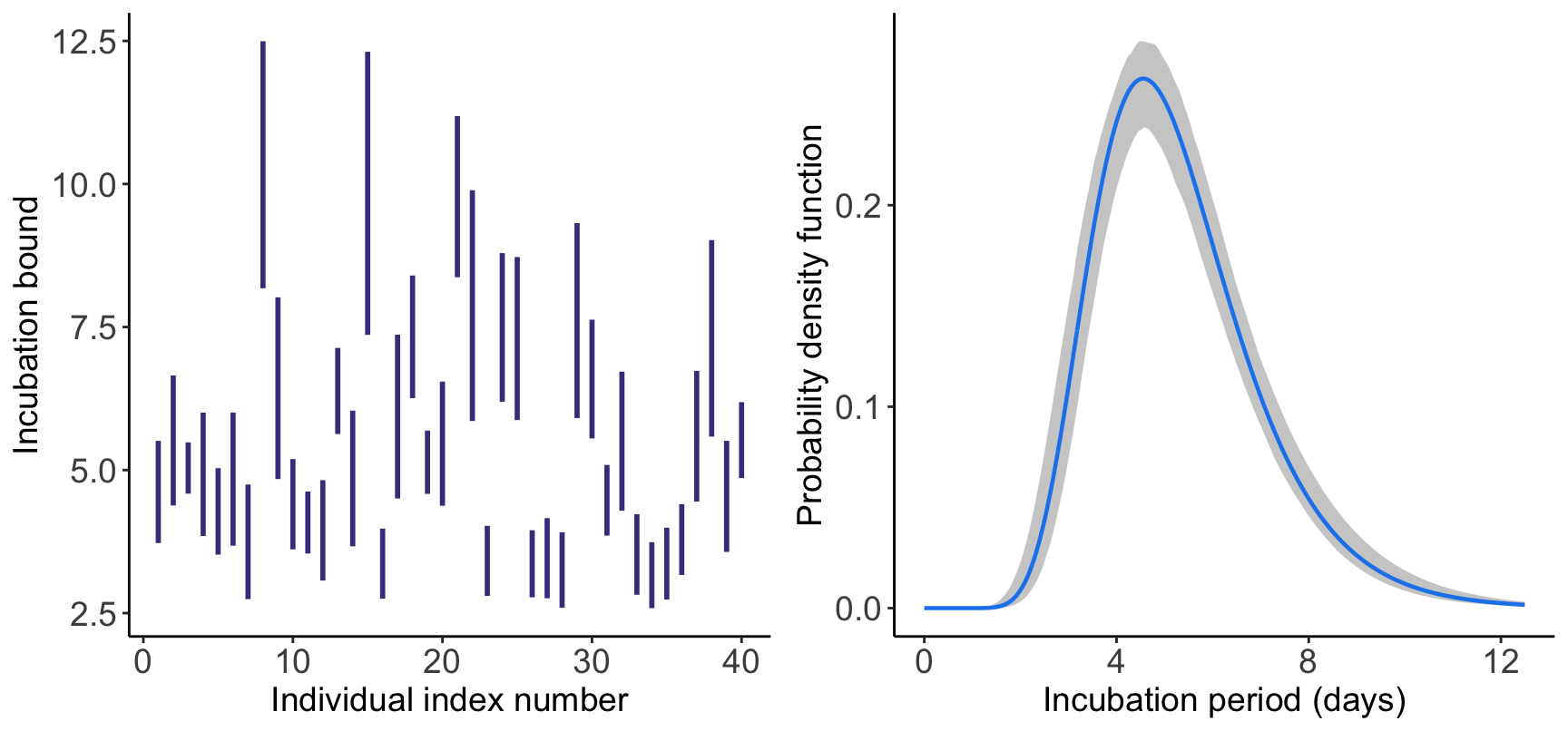
Let’s start with a simple example where x is simulated based on a data generating mechanism assuming a known incubation distribution. This can be achieved with the incubsim() routine in EpiLPS. We choose x to be generated according to a Lognormal incubation distribution with a mean of 5.5 days and a standard deviation of 2.1 days following Ferretti et al. (2020). Simulation of \(n=40\) observations with an average exposure window of 2 days is implemented as follows:
set.seed(2024)
simdat <- incubsim(incubdist = "LogNormal", n = 40, coarseness = 2)
gt(head(simdat$Dobsincub, 5))| tL | tR |
|---|---|
| 3.724500 | 5.510304 |
| 4.381377 | 6.654224 |
| 4.588020 | 5.483614 |
| 3.847835 | 6.003948 |
| 3.522282 | 5.033487 |
By typing simdat$Dobsincub, the user has access to the generated incubation intervals (expressed in days), corresponding here to a data frame with two columns and \(n=40\) rows. This is the data frame that is injected in the estimIncub() routine:
fit <- estimIncub(x = simdat$Dobsincub, verbose = TRUE)## ----------------------------------------------------------------
## Time elapsed: 1.339 seconds.
## Fitted density is Log-Normal with meanlog=1.617 and sdlog=0.317.
## Mean incubation period (days): 5.298 with 95% CI: 5.086-5.615.
## 95th percentile (days): 8.484 with 95% CI: 8.121-9.089.
## ----------------------------------------------------------------The output in the R console can easily be interpreted. It tells us that the model chooses a Lognormal density fit for the incubation period with a mean of 5.3 days (95% CI: 5.0-5.6 days). More detailed summary statistics are accessible by typing fit$stats, such as the posterior standard deviation and additional percentiles. What happens under the hood? Basically, the model computes a semi-parametric fit to the data and compares it with classic parametric fits (Lognormal, Weibull and Gamma) used for incubation modeling. The candidate with the lowest Bayesian information criterion (BIC) wins the game and is finally selected (here the Lognormal distribution). The incubation windows and the fitted incubation density can be obtained by typing:
grid.arrange(plot(fit, typ = "incubwin"), plot(fit, type = "pdf"), nrow = 1)
Real data example
The flexible Bayesian methodology is illustrated on SARS-CoV-2 symptom onset and exposure window data extracted from cases in Vietnam. The dataset was analyzed in Bui et al. (2020) and is publicly available on the GitHub repository provided in the article (https://github.com/longbui/Covid19IncubVN; last accessed July 17, 2024). The dataset contains information about \(n=19\) cases identified from January 23, 2020 to April 13, 2020. After continuity corrections (required to change calendar dates into continuous time points), the left and right incubation bounds are given by:
# Left incubation bound
tL <- c(0.504, 2.983, 5.343, 6.969, 6.990, 2.570, 6.870, 1.263, 0.693, 1.869, 1.151, 2.748, 1.209, 1.161, 4.982, 4.017, 2.170, 9.805, 1.659)

# Right incubation bound
tR <- c(1.491, 7.762, 11.777, 12.821, 11.359, 8.551, 24.954, 4.144, 6.408, 7.083, 4.191, 10.326, 9.942, 7.254, 12.690, 10.825, 14.478, 16.592, 18.649)

# Data set
dataVietnam <- data.frame(tL = tL, tR = tR)
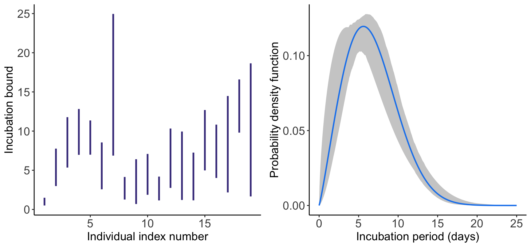
The estimIncub() routine provides a Weibull fit with a mean incubation period of 6.7 days (95% CI: 5.8-7.4 days) and the standard deviation (extracted by typing incubfit$stats) is 3.3 days (95% CI: 3.0-3.8 days). A figure of the incubation windows and the fitted Weibull density (with 95% credible interval) is also provided.
set.seed(2024)
incubfit <- EpiLPS::estimIncub(x = dataVietnam, verbose = TRUE, tmax = 25)
## ----------------------------------------------------------------
## Time elapsed: 1.13 seconds.
## Fitted density is Weibull with shape=2.142 and scale=7.521.
## Mean incubation period (days): 6.661 with 95% CI: 5.753-7.375.
## 95th percentile (days): 12.552 with 95% CI: 11.931-14.087.
## ----------------------------------------------------------------grid.arrange(plot(incubfit, typ = "incubwin"), plot(incubfit, type = "pdf"), nrow = 1)
References
Gressani, O., Torneri, A., Hens, N. and Faes, C. (2024). Flexible Bayesian estimation of incubation times. American Journal of Epidemiology (Accepted manuscript). https://doi.org/10.1093/aje/kwae192
Gressani, O., Wallinga, J., Althaus, C. L., Hens, N. and Faes, C. (2022). EpiLPS: A fast and flexible Bayesian tool for estimation of the time-varying reproduction number. PLoS Comput Biol 18(10): e1010618. https://doi.org/10.1371/journal.pcbi.1010618
Eddelbuettel, D. and Francois, R. (2011). Rcpp: Seamless R and C++ Integration. Journal of Statistical Software, 40(8), 1–18. https://doi.org/10.18637/jss.v040.i08
Ferretti, L. et al. (2020). Quantifying SARS-CoV-2 transmission suggests epidemic control with digital contact tracing. Science 368, eabb6936. https://doi.org/10.1126/science.abb6936
Bui LV, Nguyen HT, Levine H, Nguyen HN, Nguyen T-A, Nguyen TP, et al. (2020) Estimation of the incubation period of COVID-19 in Vietnam. PLoS ONE 15(12): e0243889. https://doi.org/10.1371/journal.pone.0243889
Liked this post?
- Get updates every time a new article is published (no spam and unsubscribe anytime)
- Support the blog
- Share on:


