Why this post matters

Neural networks in R are no longer niche. Today, we can choose among:

• {nnet} for classic, small-scale neural nets,
• {neuralnet} another classic neural nets package besides {nnet},
• {keras} / {keras3} for the Keras API (typically with Python backends such as TensorFlow/JAX/Torch),
• {torch} for native-R deep learning with explicit model and training control.

So why discuss another package?

In our experience, many day-to-day projects sit in the middle: we want more flexibility than a classical model, but less boilerplate than writing a full {torch} training loop. {kindling} is designed for that middle ground.

In this article, we focus on what {kindling} does well, where it helps, and where it is still limited.

What problem {kindling} solves (and what it does not)

{kindling} is a higher-level interface built on top of {torch}. In practice, it reduces repetitive code for:

• defining common network architectures,
• training feedforward and recurrent models,
• integrating with {tidymodels} ({parsnip}, {recipes}, {workflows}, {tune}).

It does not replace low-level {torch} for highly customized research code, and it does not make hardware setup disappear. You still need a working LibTorch installation and an environment that can use CPU/GPU properly.

At the time of writing (CRAN version 0.2.0), core built-in architectures include FFNN/MLP and recurrent variants (RNN/LSTM/GRU).

Setup

Install this package in two different ways:

1. Solely install {kindling} (as it installs the package dependencies internally)

install.packages("kindling")

2. You can install the package dependencies separately:

install.packages(c(
  "kindling",
  # dependencies
  "torch", "dplyr", "rsample", "recipes", "yardstick",
  "workflows", "parsnip", "tibble", "ggplot2", "mlbench", "vip"
))

Then load the packages in two ways:

1. Using library() traditionally:

library(kindling)
library(torch)
library(dplyr)
library(rsample)
library(recipes)
library(yardstick)
library(workflows)
library(parsnip)
library(tibble)
library(ggplot2)
library(mlbench)
library(vip)

In this article, we use library() for clarity and copy-paste reproducibility.

2. If you prefer a module-based and more explicit import style, use box::use() (read Box: Placing module system into R for more details).

Here’s the equivalent code as above:

box::use(
kindling[...],
dplyr[...],
rsample[...],
recipes[...],
yardstick[...],
workflows[...],
parsnip[...],
tibble[...],
ggplot2[...],
mlbench[...],
vip[...]
)

{kindling} uses {torch} as backend, so LibTorch must be installed once:

if (!torch::torch_is_installed()) {
  torch::install_torch()
}

Three levels of interaction

{kindling} is useful because you can work at different abstraction levels. Here are three ways to interact with the package, ordered from lowest to highest level of abstraction:

ffnn_generator(
  nn_name = "MyNet",
  hd_neurons = c(64, 32, 16),
  no_x = 10,
  no_y = 1,
  activations = act_funs(
    relu,
    "softplus(beta = 0.5)",
    selu
  )
)

## torch::nn_module("MyNet", initialize = function () 
## {
##     self$fc1 = torch::nn_linear(10, 64, bias = TRUE)
##     self$fc2 = torch::nn_linear(64, 32, bias = TRUE)
##     self$fc3 = torch::nn_linear(32, 16, bias = TRUE)
##     self$out = torch::nn_linear(16, 1, bias = TRUE)
## }, forward = function (x) 
## {
##     x = self$fc1(x)
##     x = torch::nnf_relu(x)
##     x = self$fc2(x)
##     x = torch::nnf_softplus(x, beta = 0.5)
##     x = self$fc3(x)
##     x = torch::nnf_selu(x)
##     x = self$out(x)
##     x
## })

mini_direct <- ffnn(
  mpg ~ .,
  data = mtcars,
  hidden_neurons = 8,
  activations = act_funs(relu),
  epochs = 20,
  verbose = FALSE
)

predict(mini_direct, newdata = head(mtcars, 3))

## [1] 11.21900 11.21385 10.56841

mini_spec <- mlp_kindling(
  mode = "regression",
  hidden_neurons = 8,
  activations = act_funs(relu), # or just "relu"
  epochs = 20,
  verbose = FALSE
)

mini_wf <- workflow() |>
  add_formula(mpg ~ .) |>
  add_model(mini_spec)

mini_fit <- fit(mini_wf, data = mtcars)

predict(mini_fit, new_data = head(mtcars, 3))

## # A tibble: 3 × 1
##   .pred
##   <dbl>
## 1 -3.49
## 2 -3.50
## 3 -3.50

Example 1: Iris classification with reproducible good practice

This first example uses direct training with ffnn(), but still follows practical steps:

• train/test split,
• feature scaling,
• validation split during training,
• regularization,
• out-of-sample evaluation.

data(iris)

iris_split <- initial_split(iris, prop = 0.8, strata = Species)
iris_train <- training(iris_split)
iris_test <- testing(iris_split)

iris_recipe <- recipe(Species ~ ., data = iris_train) |>
  step_normalize(all_predictors())
iris_prep <- prep(iris_recipe, training = iris_train)
iris_train_processed <- bake(iris_prep, new_data = NULL)
iris_test_processed <- bake(iris_prep, new_data = iris_test)

set.seed(20260218)

iris_mlp <- ffnn(
  Species ~ .,
  data = iris_train_processed,
  hidden_neurons = c(32, 16),
  activations = act_funs(relu, "softplus(beta = 0.5)"),
  loss = "cross_entropy",
  optimizer = "adam",
  learn_rate = 0.01,
  penalty = 1e-4,
  mixture = 0,
  batch_size = 16,
  epochs = 200,
  validation_split = 0.2,
  verbose = FALSE
)

iris_mlp

## 
## ======================= Feedforward Neural Networks (MLP) ======================
## 
## 
## -- FFNN Model Summary ----------------------------------------------------------
## 
## 
## -------------------------------------------------------------------------------------
##   NN Model Type           :             FFNN    n_predictors :                    4
##   Number of Epochs        :              200    n_response   :                    3
##   Hidden Layer Units      :           32, 16    reg.         :   [λ = 1e-04, α = 0]
##   Number of Hidden Layers :                2    Device       :                  mps
##   Pred. Type              :   classification                 :                     
## -------------------------------------------------------------------------------------
## 
## 
## 
## -- Activation function ---------------------------------------------------------
## 
## 
##                -------------------------------------------------
##                  1st Layer {32}    :                      relu
##                  2nd Layer {16}    :      softplus(beta = 0.5)
##                  Output Activation :   No act function applied
##                -------------------------------------------------

iris_pred <- predict(iris_mlp, newdata = iris_test_processed, type = "response")

iris_eval <- tibble(
  truth = iris_test_processed$Species,
  .pred_class = iris_pred
)

metrics(iris_eval, truth = truth, estimate = .pred_class)

## # A tibble: 2 × 3
##   .metric  .estimator .estimate
##   <chr>    <chr>          <dbl>
## 1 accuracy multiclass     0.933
## 2 kap      multiclass     0.9

conf_mat(iris_eval, truth = truth, estimate = .pred_class)

##             Truth
## Prediction   setosa versicolor virginica
##   setosa         10          0         0
##   versicolor      0          9         1
##   virginica       0          1         9

Example 2: A more realistic tabular benchmark (Sonar)

Iris is useful for teaching, but sometimes considered (too) easy. The Sonar dataset (60 numeric predictors, binary outcome) is a better stress test for tabular classification.

data("Sonar", package = "mlbench")

sonar <- Sonar |>
  mutate(Class = factor(Class))

sonar_split <- initial_split(sonar, prop = 0.8, strata = Class)
sonar_train <- training(sonar_split)
sonar_test <- testing(sonar_split)

Now fit through {tidymodels} so preprocessing and modeling stay in one pipeline:

sonar_rec <- recipe(Class ~ ., data = sonar_train) |>
  step_normalize(all_predictors())

sonar_spec <- mlp_kindling(
  mode = "classification",
  hidden_neurons = c(64, 32),
  activations = act_funs(relu, relu),
  optimizer = "adam",
  learn_rate = 0.001,
  penalty = 1e-4,
  mixture = 0,
  batch_size = 16,
  epochs = 250,
  validation_split = 0.2,
  verbose = FALSE
)

sonar_wf <- workflow() |>
  add_recipe(sonar_rec) |>
  add_model(sonar_spec)

set.seed(20260218)
sonar_fit <- fit(sonar_wf, data = sonar_train)

sonar_pred <- augment(sonar_fit, new_data = sonar_test)

metrics(sonar_pred, truth = Class, estimate = .pred_class)

## # A tibble: 2 × 3
##   .metric  .estimator .estimate
##   <chr>    <chr>          <dbl>
## 1 accuracy binary         0.837
## 2 kap      binary         0.672

In practice, this setup is often a strong baseline for tabular binary classification before trying larger architectures.

About early stopping and callbacks

If you come from Keras/TensorFlow, you may be used to callback objects (early stopping, learning-rate schedules, etc.).

With {kindling} 0.2.0, practical overfitting control is usually handled through:

• validation_split,
• regularization (penalty, mixture),
• tuning model size and training length (epochs),
• proper resampling with {tidymodels}.

In other words, we can approximate early-stopping behavior by selecting epochs via validation/resampling, even without a callback-heavy workflow.

Supported architectures (current scope)

Variable importance (FFNN)

Interpretability for neural networks is imperfect, but {kindling} integrates established approaches for FFNN models.

# For FFNN fits:
garson(iris_mlp, bar_plot = FALSE)

##        x_names y_names  rel_imp
## 1 Petal.Length       y 33.39467
## 2  Sepal.Width       y 24.44282
## 3  Petal.Width       y 21.92705
## 4 Sepal.Length       y 20.23546

olden(iris_mlp, bar_plot = FALSE)

##        x_names y_names    rel_imp
## 1 Petal.Length       y -2.4176215
## 2  Petal.Width       y -1.8339908
## 3 Sepal.Length       y -0.6675719
## 4  Sepal.Width       y  0.5844613

# Via vip (Olden/Garson methods supported by kindling S3 methods)
vi(iris_mlp, type = "olden") |>
  vip()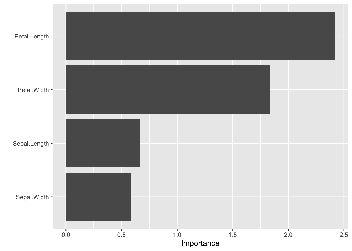

We recommend using these as directional diagnostics, not as causal evidence.

When {kindling} is a good fit

{kindling} is a practical choice when our projects:

• work mostly in R and want to stay inside {tidymodels},
• need neural nets for tabular or moderate sequence tasks,
• want less boilerplate than raw {torch} but still meaningful control.

It may be less ideal when our projects need:

• custom research architectures and training loops,
• mature callback ecosystems similar to high-level Keras workflows,
• highly optimized distributed production pipelines.

Limitations to keep in mind

• Hardware setup still matters: GPU usage depends on a correct {torch}/LibTorch installation and supported hardware.
• Ecosystem maturity: this is a young package; interfaces can evolve.
• Debugging depth: for deeply custom debugging, low-level {torch} remains the reference path.
• Model class assumptions: recurrent models are for sequence-structured data; using them on plain tabular data is usually not appropriate.

Takeaways

{kindling} is not about replacing {torch} or {keras3}. It is about reducing friction for common deep-learning workflows in R.

For many applied projects, a robust pattern is:

1. preprocess with {recipes},
2. start with a modest MLP architecture,
3. use validation split + regularization,
4. evaluate on held-out test data,
5. tune only after you have a strong baseline.

If this matches your workflow, {kindling} is worth trying.

As always, if you have any question related to the topic covered in this post, please add it as a comment so other readers can benefit from the discussion.